Everything below is in the live script. Run it line by line at home, as many times as it takes.
Objectives
By the end of this session you can:
Build, index and combine matrices.
Build and index lists, and tell [ from [[.
Run one function over every row, column, group or file.
Read a real CSV, fix its types, and write results back out.
Join two tables, and check the row count before and after.
Matrices
A matrix is one vector with dimensions.
m <-matrix(1:6, nrow =2)m
#>      [,1] [,2] [,3]
#> [1,]    1    3    5
#> [2,]    2    4    6
c(dim(m), nrow(m), ncol(m))
#> [1] 2 3 2 3
matrix(1:6, nrow =2, byrow =TRUE) # filled across, not down
#>      [,1] [,2] [,3]
#> [1,]    1    2    3
#> [2,]    4    5    6
matrix(1:2, nrow =2, ncol =3) # too few values: R recycles them
#>      [,1] [,2] [,3]
#> [1,]    1    1    1
#> [2,]    2    2    2
R folds the vector down the columns unless you say byrow = TRUE. Get that backwards and every value lands in the wrong cell, with no error.
The last line is the one that bites. Give matrix() fewer values than cells and it recycles them to fill the shape, silently, as long as the count divides evenly. When it does not divide evenly you get a warning, which is the friendlier case. Check dim() against what you meant.
Indexing a matrix
m[2, 3] # row 2, column 3
#> [1] 6
m[2, ] # all of row 2
#> [1] 2 4 6
m[, 3] # all of column 3
#> [1] 5 6
class(m[, 3]) # a plain vector: the dimension was dropped
#> [1] "integer"
class(m[, 3, drop =FALSE]) # still a matrix
#> [1] "matrix" "array"
head(m, 1) # first rows; tail() for the last
#>      [,1] [,2] [,3]
#> [1,]    1    3    5
Two coordinates, m[row, column], and a blank means all of them. The same rule you use on a data frame.
Note that m[2, ] came back as a plain vector, not a one-row matrix. R drops the dimension when you ask for a single row or column, which is convenient at the console and a bug inside a function that expected a matrix. drop = FALSE keeps the shape.
#>         Jan Feb Mar
#> Compton  12  15  19
#> Reseda   14  17  22
temps["Reseda", "Feb"] # by name, not position
#> [1] 17
temps[, c("Jan", "Feb")] # several at once
#>         Jan Feb
#> Compton  12  15
#> Reseda   14  17
temps[temps >15] # by logical: returns a vector
#> [1] 17 19 22
Three notations, one operation. Position counts, names read, and a logical test picks whatever passes.
Names are worth setting the moment a matrix means something. temps[2, 2] is a number you have to decode; temps["Reseda", "Feb"] says what it is, and it keeps working when the rows get reordered.
The logical form behaves differently from the other two: it hands back a plain vector, not a matrix, because the cells that pass do not generally form a rectangle. Ask for the positions instead with which(temps > 15, arr.ind = TRUE) when you need to know where they were.
diag() does two jobs depending on what you hand it. Give it a matrix and it extracts the diagonal. Give it a single number and it builds an identity matrix of that size. Give it a vector and it builds a diagonal matrix with that vector down the middle and zeros elsewhere.
Diagonal matrices come up constantly once you write estimators by hand: weights, variances, and the identity that sits in a projection formula are all diagonal. Most of a diagonal matrix is zeros, which is worth remembering for later today.
Matrix arithmetic
temps *9/5+32# every cell at once, Celsius to Fahrenheit
#>          Jan  Feb  Mar
#> Compton 53.6 59.0 66.2
#> Reseda  57.2 62.6 71.6
t(temps) # flip rows and columns
#>     Compton Reseda
#> Jan      12     14
#> Feb      15     17
#> Mar      19     22
Arithmetic runs cell by cell, exactly as it does on a vector, because underneath a matrix is a vector.
This is why images and grids are stored as matrices. A photograph is a matrix of pixel values, and making it brighter is one multiplication. A weather grid is a matrix of temperatures, and converting the whole grid to Fahrenheit is the line above.
Combining matrices
more <-matrix(c(9, 11, 16), nrow =1,dimnames =list("Pasadena", c("Jan", "Feb", "Mar")))rbind(temps, more) # a new row: same columns
#>          Jan Feb Mar
#> Compton   12  15  19
#> Reseda    14  17  22
#> Pasadena   9  11  16
cbind(temps, Apr =c(21, 24)) # a new column: same rows
#>         Jan Feb Mar Apr
#> Compton  12  15  19  21
#> Reseda   14  17  22  24
Matrix::bdiag(diag(2), matrix(1, 2, 2)) # blocks down the diagonal
rbind() stacks matrices on top of each other and cbind() puts them side by side. The shared margin has to agree: rbind() needs the same number of columns, cbind() the same number of rows.
R matches columns by position, not by name. If the second matrix carries the same three months in a different order, rbind() will stack them anyway and put February’s numbers under the January heading, with no warning. Check the names agree before you stack, not after.
One vector underneath means one class throughout. Add a row of text and every number becomes text, silently, with no warning. It is the same conversion that turns a numeric column into text when one entry is a word.
A data frame does not do this, because its columns are separate vectors. That is the whole reason both containers exist: tables of mixed data are data frames, and grids of one measurement are matrices.
Sparse matrices
Most of the cells are zero. Store only the ones that are not, and both the memory and the arithmetic get cheaper.
library(Matrix)set.seed(1); n <-2000d <-matrix(0, n, n); d[sample(n * n, n * n *0.01)] <-1# 1% non-zeros <-Matrix(d, sparse =TRUE); v <-rnorm(n)c(dense =format(object.size(d), units ="MB"),sparse =format(object.size(s), units ="MB"))
#>     dense    sparse
#> "30.5 Mb"  "0.5 Mb"
c(dense =system.time(for (i in1:20) d %*% v)[["elapsed"]],sparse =system.time(for (i in1:20) s %*% v)[["elapsed"]])
#>  dense sparse
#>  0.072  0.004
A dense matrix stores every cell, including all the zeros. A sparse matrix stores only the non-zero values and the positions they sit in. Same numbers, same indexing, a fraction of the memory.
The arithmetic gets faster too, which is the part that pays. Multiplying skips the zeros instead of multiplying by them, so the same product runs more than ten times quicker here. Two things you will do constantly are matrix multiplications underneath: aggregating values up to groups, which is a matrix of weights times a vector of values, and any estimator written in matrix form.
You meet these the moment a matrix gets large and mostly empty: a county-by-county adjacency matrix, a word-by-document count, a design matrix of fixed effects with one 1 per row, or extraction weights mapping grid cells to regions. At n = 2000 the saving is a convenience. At n = 100,000 it decides whether the code runs at all.
Matrix ships with R, so there is nothing to install. Its matrices index and multiply like ordinary ones; as.matrix() converts back when a function insists on dense input.
Lists
A list holds anything, in any mix, at any length.
l <-list(site ="Compton", readings =c(53.2, 33.6, 47.0), clean =TRUE)str(l)
#> List of 3
#>  $ site    : chr "Compton"
#>  $ readings: num [1:3] 53.2 33.6 47
#>  $ clean   : logi TRUE
length(l) # three elements...
#> [1] 3
lengths(l) # ...of these lengths
#>     site readings    clean
#>        1        3        1
Text, a numeric vector, and a logical, side by side in one object. A vector could not do this: it would convert everything to text. A matrix could not either: one type throughout, and every row the same length.
That freedom is the point. Lists are what R uses whenever the pieces do not line up.
Single and double brackets
l["readings"] # a LIST of length one
#> $readings
#> [1] 53.2 33.6 47.0
l[["readings"]] # the vector itself
#> [1] 53.2 33.6 47.0
l$readings # the same thing, less typing
#> [1] 53.2 33.6 47.0
class(l["readings"])
#> [1] "list"
class(l[["readings"]])
#> [1] "numeric"
The mistake to expect is arithmetic on a single-bracket result: mean(l["readings"]) fails, because you handed mean() a list. $ and [[ ]] do the same job; [[ ]] is the one that also takes a variable, which matters as soon as the name is computed rather than typed.
A list is a chest of drawers
Think of the list as a chest of drawers. Single brackets take the drawer out of the chest, and a drawer is still a drawer. Double brackets open the drawer and hand you what is inside.
#> List of 3
#>  $ id  : chr "060371302"
#>  $ site:List of 3
#>   ..$ name: chr "Compton"
#>   ..$ lat : num 33.9
#>   ..$ lon : num -118
#>  $ pm  : num [1:3] 53.2 33.6 47
An element of a list can be another list, to any depth. Chain the operators to walk down: $ after $, or [[ ]] after [[ ]].
This is exactly the shape of the JSON that web APIs return, which is why the lesson pays off well beyond R. str() is how you find your way around one you did not build.
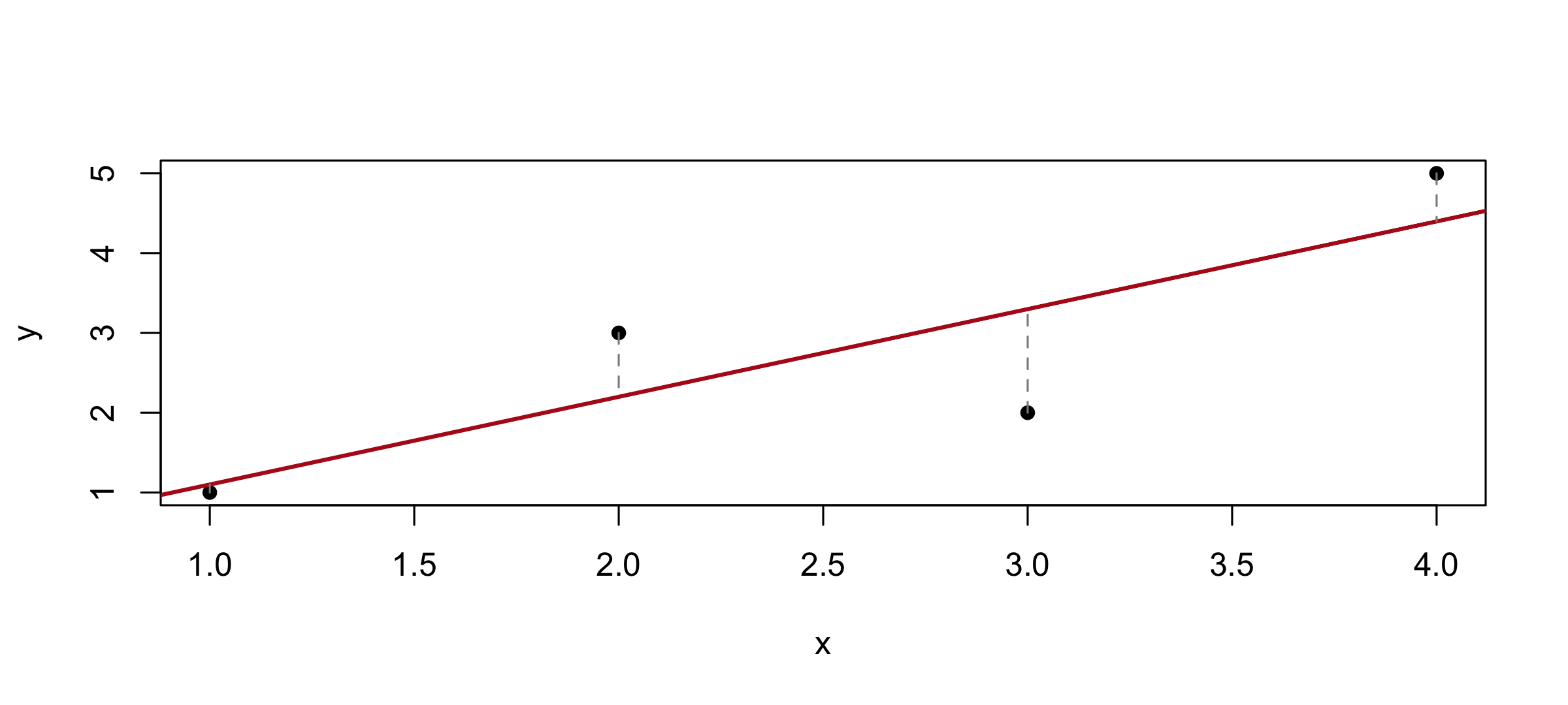
plot(x, y, pch =16, xlab ="x", ylab ="y")abline(fit, col ="#b31b1b", lwd =2)segments(x, y, x, fitted(fit), lty =2, col ="grey55") # the residuals
Most functions that return more than one thing return a list, because a list is the only container that can hold a number, a vector and a data frame at once.
A fitted model is a list with a class on it. names() shows you the parts and $ takes one out. Every modelling function you meet this semester follows this pattern, so knowing lists means never being stuck at “what did this thing give me?”
The plot is what those numbers describe. fit$coefficients is the line, fitted(fit) is where the line sits above each x, and fit$residuals is the length of each dashed segment. Three elements of one list, all visible at once.
Combining list elements
pieces <-list(a =c(1, 2), b =c(3, 4), c =c(5, 6))unlist(pieces) # one flat vector, names kept
#> a1 a2 b1 b2 c1 c2
#>  1  2  3  4  5  6
do.call(rbind, pieces) # one matrix, one row per element
#>   [,1] [,2]
#> a    1    2
#> b    3    4
#> c    5    6
unlist() flattens a list into a single vector. It is convenient and it is lossy: everything becomes one type, and any structure below the top level disappears.
do.call(f, list) calls f with the list’s elements as its arguments, so do.call(rbind, pieces) is rbind(pieces$a, pieces$b, pieces$c) without your having to know how many there are or what they are called. That is the standard way to turn a list of rows into a matrix, or a list of data frames into one data frame.
# 1. Build a diagonal matrix with the numbers 1 to 5 down the middle.## 2. From m (the 2 x 3 matrix), pull the second column two ways: once# as a vector, once still a matrix.## 3. l["readings"] and l[["readings"]]: which one can you take a mean of?# Find out with class(), not from memory.
class(l["readings"]); class(l[["readings"]]) # list vs numeric
#> [1] "list"
#> [1] "numeric"
apply(): over rows and columns
You built these containers and picked things out of them. Now the other half: run one function over every row, column, group or file.
apply(temps, 1, mean) # 1 = rows
#>  Compton   Reseda
#> 15.33333 17.66667
apply(temps, 2, mean) # 2 = columns
#>  Jan  Feb  Mar
#> 13.0 16.0 20.5
rowMeans(temps); colMeans(temps) # same answers, named and faster
#>  Compton   Reseda
#> 15.33333 17.66667
#>  Jan  Feb  Mar
#> 13.0 16.0 20.5
rowSums(temps)
#> Compton  Reseda
#>      46      53
apply(m, MARGIN, f) runs f over one margin of a matrix and collects the results.
The margin numbers are the bracket coordinates. You write m[row, column], so 1 is rows and 2 is columns. Margin 1 gives you one answer per row; margin 2 gives you one per column.
rowMeans() and colMeans() are fast special cases of exactly this.
apply() with any function
apply(temps, 2, max)
#> Jan Feb Mar
#>  14  17  22
apply(temps, 2, range) # two numbers per column
#>      Jan Feb Mar
#> [1,]  12  15  19
#> [2,]  14  17  22
apply(temps, 2, function(x) max(x) -min(x)) # write your own, inline
#> Jan Feb Mar
#>   2   2   3
The function is an argument like any other. Pass it by name with no parentheses, or write it inline with function(x) when it is too small to deserve a name. Inside, x is one row or one column.
range returns two numbers per column, so apply() hands back a matrix rather than a vector. What you get out depends on what your function returns.
split() cuts an object into a list, one element per group. Those are the same six numbers that went into temps, arranged as a list of two vectors instead of a two-row matrix.
That is the choice in miniature. A matrix needs every group to be the same length; a list does not. Real groups are rarely the same size, which is why split() returns a list.
lapply(x, f) runs f on every element of x and returns a list of the same length, with the same names. One call, one result per group, and no loop written by hand.
Inside the function, the argument is one element: here, one site’s readings. You write the code once, for one group, and lapply() handles the repetition.
sapply(): the same, simplified
sapply(by_site, mean) # a named vector, not a list
#>  Compton   Reseda
#> 15.33333 17.66667
sapply(by_site, length)
#> Compton  Reseda
#>       3       3
sapply(by_site, range) # two numbers each, so a matrix comes back
#>      Compton Reseda
#> [1,]      12     14
#> [2,]      19     22
apply(temps, 1, mean) # same answers, from the matrix
#>  Compton   Reseda
#> 15.33333 17.66667
sapply() is lapply() plus one step: when every result is a single value, it returns a named vector instead of a list. When every result is the same longer length, it returns a matrix.
Use sapply() when you want something to print or compute with. Use lapply() when each result is bigger than one value, or when you want the shape guaranteed. sapply() decides what to return based on what it gets, which is convenient at the console and a hazard inside a script.
The last line is the same question asked of the matrix. Two containers, two verbs, one answer: apply() walks a margin, sapply() walks a list.
# 1. One line: the highest reading in each city. One line: the highest# in each month.## 2. One line: the range of each site in by_site. Why does that come# back as a matrix?
dim(sapply(by_site, range)) # ...so sapply stacks them into a matrix
#> [1] 2 2
Reading a CSV
la <-read.csv("data/epa_pm25_la_county_2025.csv")dim(la)
#> [1] 4757 22
# Uncomment and run once. Same file, fetched instead of clicked.# dir.create("data", showWarnings = FALSE)# download.file(paste0("https://arielortizbobea.github.io/aem6850/",# "fall-2026/sessions/data/epa_pm25_la_county_2025.csv"),# "data/epa_pm25_la_county_2025.csv")
read.csv() takes a path relative to the working directory, which getwd() prints and list.files() lets you check. “File not found” is almost always a disagreement about where you are, not a missing file.
4,757 rows and 22 columns: every monitor in the county, every day of 2025.
A data frame is a list of columns
is.list(la) # a data frame IS a list
#> [1] TRUE
length(la) # of 22 columns
#> [1] 22
head(sapply(la, class)) # so sapply walks the columns
#>                           Date                         Source
#>                    "character"                    "character"
#>                        Site.ID                            POC
#>                      "integer"                      "integer"
#> Daily.Mean.PM2.5.Concentration                          Units
#>                      "numeric"                    "character"
A data frame is a list of equal-length vectors with a class on top. $ is the list’s own operator, which is why the same notation reaches a column of a table and an element of a list.
That is why sapply() works here with no extra effort: hand it a data frame and it walks the columns. On a file with 22 columns this beats scrolling through str() output, and it puts two problems on screen at once. Site.ID came in as an integer. Date came in as character.
Identifiers read as numbers
la$Site.ID[1] # what R holds
#> [1] 60370016
The file says 060370016. R says 60370016.
read.csv() looked at a column of digits and decided it was a number, and the leading zero of a number is meaningless, so it is gone. The identifier is now wrong, silently, and it will fail to match every other file that spells it correctly.
This is not an EPA quirk. FIPS codes, ZIP codes, CUSIPs, phone numbers and account numbers all lead with zeros that R will strip on the way in.
colClasses: setting types at read time
la <-read.csv("data/epa_pm25_la_county_2025.csv",colClasses =c("Site.ID"="character"))la$Site.ID[1]
length(unique(la$Site.ID)) # ...so this counts monitors: eleven
#> [1] 11
colClasses names the columns you want read a particular way. Everything you do not name is guessed as before.
Fix it at read time, not afterwards. Once the zero is gone, as.character() gives you back "60370016", which is a different string from "060370016" and matches nothing. The information left the building when the file came in.
Dates
la$Date[1]
#> [1] "01/01/2025"
class(la$Date)
#> [1] "character"
la$date <-as.Date(la$Date, format ="%m/%d/%Y")class(la$date)
#> [1] "Date"
range(la$date)
#> [1] "2025-01-01" "2025-12-31"
Pulling pieces out of a date
d <-as.Date("2025-01-07")c(month =format(d, "%m"), name =format(d, "%b"),year =format(d, "%Y"), doy =format(d, "%j"),day =weekdays(d))
#>     month      name      year       doy       day
#>      "01"     "Jan"    "2025"     "007" "Tuesday"
la$month <-format(la$date, "%m")
format() runs the parsing backwards: give it a code and it returns that piece as text. weekdays() and months() are the two shortcuts worth remembering, because they are what you want for seasonality and for day-of-week effects.
%m/%d/%Y is a format string describing where the pieces are:
Dates are numbers
d +30# thirty days later
#> [1] "2025-02-06"
as.Date("2025-03-01") - d # how far apart
#> Time difference of 53 days
seq(d, by ="week", length.out =4) # a sequence of dates
Underneath, a Date is a count of days since January 1, 1970. That is why + and - work, why seq() can step by "day", "week", "month" or "year", and why sorting finally puts dates in time order. Text dates sort character by character, so "10/01" lands before "9/01".
Two-digit month, slash, two-digit day, slash, four-digit year. Get a code wrong and you get NAs rather than an error, so check range() afterwards.
Checking for duplicate rows
Before averaging anything, find out what one row is.
key <- la[, c("Site.ID", "date")]anyDuplicated(key) # 0 means none; otherwise the first repeated row
#> [1] 695
sum(duplicated(key)) # how many rows repeat a site-day
#> [1] 1270
frm <- la[la$AQS.Parameter.Code ==88101& la$POC ==1, ]anyDuplicated(frm[, c("Site.ID", "date")]) # 0: one row per site-day now
#> [1] 0
duplicated() returns TRUE for every row that repeats an earlier one, so sum() counts them. anyDuplicated() is the fast version: it stops at the first repeat and returns its position, or 0 if the rows are unique. Use anyDuplicated() when you want a yes or no, and duplicated() when you want to see the offenders: key[duplicated(key), ].
There are 1,270 repeated site-days here. Nothing warned you: the file is correct, it just is not one row per thing you think you are counting.
The reason is that a site can run several instruments, and the file gives each its own row on the same day. Take a mean now and you average a site with itself, weighted by how many instruments it happens to run. That is not a number about air quality; it is a number about equipment.
The fix keeps one instrument per site. Parameter 88101 is the federal reference method, and POC == 1 takes the first instrument at each site. Then the check passes, and every row is one site on one day.
Ask this of every file. “What is one row?” is the question that catches duplicated keys, and it is the same check a join needs later.
tapply(): a matrix from two groupings
Numbers to summarise, what to group them by, a function to run on each group. Two groupings give one value per combination.
Read the call left to right. The first argument is the column you want summarised, here the concentration. The second says how to cut it up: list(site, month) means group by site and by month, so every site-and-month pair is its own group. The third is what to compute on each group, here mean.
tapply() then does three things. It splits the vector into those groups, runs the function on each one, and arranges the answers by the groupings it was given. One grouping gives a named vector. Two give a matrix, with the first grouping down the rows and the second across the columns: eight sites by twelve months, one mean in each of the 96 cells.
Cells with no rows come back NA rather than zero, which is the honest answer. A month a site never reported is missing, not clean air.
A long file of 4,757 rows is now a grid you can read at a glance. That is the move worth taking away: the data frame is how the file arrives, and the matrix is the shape the question has.
reshape(): long and wide
tapply() gave a matrix. reshape() does the same turn on a data frame, and turns it back.
#>   site month pm25
#> 1    A    01 21.3
#> 2    A    02 13.4
#> 3    B    01 11.6
#> 4    B    02  7.2
wide <-reshape(long, direction ="wide",idvar ="site", timevar ="month", v.names ="pm25")wide
#>   site pm25.01 pm25.02
#> 1    A    21.3    13.4
#> 3    B    11.6     7.2
reshape(): back to long
reshape(wide, direction ="long", idvar ="site",varying =list(2:3), v.names ="pm25", times =c("01", "02"))
#>      site time pm25
#> A.01    A   01 21.3
#> B.01    B   01 11.6
#> A.02    A   02 13.4
#> B.02    B   02  7.2
Long means one row per observation, with a column saying which group it belongs to. Wide means one row per unit and one column per group. The same numbers, two shapes, and most of the reshaping you will do in your career is moving between them.
The arguments name the pieces: idvar is what stays a row, timevar is what becomes columns, and v.names is the value being spread. Going back, varying names the columns to stack and times says what to call them.
Base reshape() is famously awkward, and it is worth knowing that tidyr::pivot_wider() and pivot_longer() do the same job with friendlier arguments. Panels arrive long, regressions usually want long, and tables for readers want wide.
apply() over both margins
round(sort(apply(tb, 1, mean), decreasing =TRUE), 1) # per site, all year
#>                        Compton  Los Angeles-North Main Street
#>                           12.9                           12.7
#>                 Pico Rivera #2 Long Beach-Route 710 Near Road
#>                           12.3                           12.3
#>                       Pasadena             Signal Hill (LBSH)
#>                           11.4                           10.7
#>                         Reseda        Lancaster - Fairgrounds
#>                            9.2                            4.5
round(apply(tb, 2, mean), 1) # per month, all sites
Read that first line from the inside out, which is how you write it too: apply(tb, 1, mean) gives one number per site, sort() puts them in order, round() tidies them for printing. Build the innermost piece, run it, look at what came back, then wrap the next call around it. Typing the whole nest in one go and hoping is how you end up debugging four functions at once.
Now the two margins answer two different questions with the same verb.
Down the rows: which monitors sit in the dirtiest air all year. Lancaster, out in the desert, reads a third of what the basin sites do.
Across the columns: what the county did month by month. January is the worst month at nearly every site at once, which is the signature of something county-wide rather than one instrument drifting.
merge(): joining two tables
Results in one table, the thing you want to attach in another. merge() matches them on a shared column.
sites <-merge(means, coords, by ="site")nrow(sites) # and after
#> [1] 8
by names the column the two tables share. Rows whose keys match are glued side by side; the result carries the columns of both.
Eight rows in, eight rows out, so nothing was lost. That check is the whole discipline of joining. Write down the row count you expect before you run it, and compare. A join has two silent failure modes and neither one errors.
How merge() drops and duplicates rows
partial <- coords[coords$site !="Compton", ] # pretend one site is missingnrow(merge(means, partial, by ="site")) # dropped
#> [1] 7
nrow(merge(means, partial, by ="site", all.x =TRUE)) # kept, with NA
#> [1] 8
Rows can disappear. By default merge() keeps only keys present in both tables, so a site missing from the lookup takes its result with it. Seven rows came back where you asked about eight, with no error and no warning. all.x = TRUE keeps every row of the first table and fills the missing side with NA, which is almost always what you want: an NA you can see beats a row you cannot.
Rows can also multiply. If the second table has two rows for one site, every matching row of the first is repeated to pair with each. Ask for eight and get twelve. That is why unique() is in the line that built coords.
Keys have to be the same type, too. A site id read as a number will not match the same id read as text, and that failure looks exactly like “no matching rows”.
list.files() gives you the names, and lapply() or sapply() runs the same call on each one.
This is the shape of most real data collection: one file per year, per state or per month, and one function that handles any single file. You get it right once, then hand the function the list. do.call(rbind, ...) on the result stacks them into one frame.
write.csv() is read.csv() run backwards. row.names = FALSE stops R adding a column of row numbers you never asked for, which is the most common complaint about files written from R. Round before you write, not after: a mean lands in the file as 19.386666666667 unless you say round(x, 1).
CSV forgets what things were. It is text, so a Date comes back as character, a factor comes back as character, and every column has to be guessed again on the way in. That is fine for a results table someone else will open, and wrong for an intermediate you will read back into R.
saveRDS() writes one R object exactly as it is, compressed. Dates stay dates, factors keep their levels, and readRDS() hands it back unchanged. Use it for anything you computed and do not want to recompute. save() and load() do the same for several objects at once, but they restore names into your workspace instead of returning a value, so saveRDS() is easier to reason about.
Other people’s formats. Applied economics runs on Stata files, and the haven package reads and writes them: read_dta(), write_dta(), plus read_sav() for SPSS and read_sas() for SAS. readxl::read_excel() opens spreadsheets, and writexl::write_xlsx() writes them. For data too big for CSV to be sensible, arrow::write_parquet() writes a columnar file that loads far faster and keeps its types.
# Everything below uses la, frm and tb, built earlier in this script.# Matrices# 1. Build a 3 x 4 matrix of the numbers 1 to 12, filled across the rows.# 2. Same matrix: what is the sum of each row? Of each column?# 3. Same matrix: divide every cell by its own column's total.# 4. Add a fourth row of zeros with rbind(). Then add a fifth column.# 5. Run rbind(c(1, 2), c("a", "b")). What class is the result, and why?# Lists# 6. Build a list holding your name, the numbers 1 to 5, and TRUE.# 7. Same list: pull the numeric vector out two different ways.# 8. What class does l["readings"] return? Check with class().# 9. Split "2025-01-07" on the dash and get back a vector of three pieces.# 10. unlist() the list from question 6. What happened to the numbers?# apply and friends# 11. Which column of la came in as character? (One line, all 22 at once.)# 12. How many rows does each site have in la? (One line.)# 13. Which month had the highest county-wide mean, and what was it?# 14. Which site had the single dirtiest month of 2025?# 15. Rebuild tb with median instead of mean. Where do the two disagree# most, and what does that tell you about those days?# 16. One line: the number of rows in every CSV in your data folder.
# 1mm <-matrix(1:12, nrow =3, byrow =TRUE)# 2apply(mm, 1, sum); apply(mm, 2, sum)# 3sweep(mm, 2, colSums(mm), "/")# 4mm <-rbind(mm, 0); mm <-cbind(mm, 0)# 5 character: one vector underneath, so one type throughoutclass(rbind(c(1, 2), c("a", "b")))# 6l3 <-list(name ="Ariel", nums =1:5, ok =TRUE)# 7l3$nums; l3[["nums"]]# 8 a list of length one, not the vector: single brackets stay wrappedclass(l["readings"])# 9strsplit("2025-01-07", "-")[[1]]# 10 everything became text: one type, and "TRUE" is now a wordunlist(l3)# 11 a data frame is a list of columns, so sapply walks themnames(which(sapply(la, class) =="character"))# 12table(la$Local.Site.Name)# 13month_means <-apply(tb, 2, mean, na.rm =TRUE)month_means[which.max(month_means)]# 14which(tb ==max(tb, na.rm =TRUE), arr.ind =TRUE)# 15 the mean sits above the median wherever a few days ran very hightb_med <-tapply(frm$Daily.Mean.PM2.5.Concentration,list(frm$Local.Site.Name, frm$month), median)round(sort(apply(tb - tb_med, 1, mean, na.rm =TRUE), decreasing =TRUE), 2)# 16sapply(list.files("data", pattern ="\\.csv$"),function(f) nrow(read.csv(file.path("data", f))))
Quick reference
Matrices
Code
What it does
matrix(x, nrow =, ncol =, byrow =)
Build one; byrow = TRUE fills across; short input is recycled
dim(m), nrow(m), ncol(m)
Its shape
m[i, j], m[i, ], m[, j]
Cell, row, column; blank means all
m[, j, drop = FALSE]
Keep it a matrix instead of dropping to a vector
rownames(m), colnames(m)
Names on the margins
m["a", "Feb"], m[, c("a", "b")]
Subset by name instead of position
m[m > 15]
Subset by logical; returns a vector, not a matrix
which(m > 15, arr.ind = TRUE)
The row and column of every cell that passes
t(m), m %*% v
Transpose; matrix multiplication
diag(m)
Pull out the diagonal
diag(3), diag(c(4, 5, 6))
Build an identity matrix; build a diagonal one
Matrix::bdiag(a, b)
Blocks down the diagonal, zeros elsewhere
rbind(a, b), cbind(a, b)
Stack; widen. Matched by position, not by name
head(m, 3), tail(m)
First or last rows; works on frames too
rowSums(m), rowMeans(m)
One number per row, fast
colSums(m), colMeans(m)
One number per column, fast
sweep(m, 2, v, "/")
Divide every column by its own entry in v
Matrix(m, sparse = TRUE)
Store only the non-zeros; library(Matrix)
object.size(x), system.time(expr)
How big it is; how long it took
Lists
Code
What it does
list(a = , b = )
Build one; anything, any length
l[["a"]], l$a
The element itself
l["a"]
A list of length one, not the element
names(l), is.list(x)
The element names; is this a list at all
str(l), lengths(l)
What is in there; how long each part is
unlist(l)
Flatten to one vector, one type
do.call(rbind, l)
Stack the elements into a matrix or frame
lm(y ~ x), fitted(fit)
A fitted model is a list; the values on the line
plot(x, y), abline(fit), segments()
Draw the points, the fitted line, the residuals
One function, many things
Code
What it does
apply(m, 1, f)
Once per row; 2 for columns
apply(m, 2, function(x) ...)
Write the function inline when it is small
split(x, g)
A list, one element per group
lapply(l, f)
A list in, a list of the same length out
sapply(l, f)
The same, simplified to a vector or matrix
tapply(x, list(g1, g2), f)
A matrix of f over two groupings
reshape(d, direction = "wide", idvar =, timevar =, v.names =)
Long to wide
reshape(d, direction = "long", varying =, v.names =, times =)
Wide back to long
sapply(d, class)
The class of every column at once
Dates
Code
What it does
as.Date(x, format = "%m/%d/%Y")
Text to a real date; wrong format gives NA, not an error
format(d, "%m"), "%b", "%Y", "%j"
Month, short month name, year, day of the year
weekdays(d), months(d)
The day and month names
d + 30, d2 - d1
Dates are numbers, so arithmetic works
seq(d, by = "week", length.out = 4)
A sequence of dates; also "day", "month", "year"
range(d), sort(d)
The span; in order
Vectors you will keep reaching for
Code
What it does
unique(x)
Drop repeats; length(unique(x)) counts distinct values
duplicated(d)
TRUE for each row that repeats an earlier one
anyDuplicated(d)
Position of the first repeat, or 0 if there are none
which.max(x), which.min(x)
The position of the extreme value
x[which.max(x)]
…so this is the value itself
max(x), min(x), range(x)
The extremes
sort(x), order(x)
Sorted values; the positions that would sort them
strsplit(x, "-")
Split text; returns a list, so [[1]] to get the pieces