AEM 6850

Empirical Methods for Applied Economists

Prof. Ariel Ortiz-Bobea

3 · R essentials II

Tuesday, September 1, 2026

Objectives

By the end of this session you can:

Build, index and combine matrices.
Build and index lists, and tell [ from [[.
Run one function over every row, column, group or file.
Read a real CSV, fix its types, and write results back out.
Join two tables, and check the row count before and after.

Matrices

A matrix is one vector with dimensions.

m <- matrix(1:6, nrow = 2)
m

#>      [,1] [,2] [,3]
#> [1,]    1    3    5
#> [2,]    2    4    6

c(dim(m), nrow(m), ncol(m))

#> [1] 2 3 2 3

matrix(1:6, nrow = 2, byrow = TRUE)   # filled across, not down

#>      [,1] [,2] [,3]
#> [1,]    1    2    3
#> [2,]    4    5    6

matrix(1:2, nrow = 2, ncol = 3)       # too few values: R recycles them

#>      [,1] [,2] [,3]
#> [1,]    1    1    1
#> [2,]    2    2    2

Indexing a matrix

m[2, 3]     # row 2, column 3

#> [1] 6

m[2, ]      # all of row 2

#> [1] 2 4 6

m[, 3]      # all of column 3

#> [1] 5 6

class(m[, 3])                # a plain vector: the dimension was dropped

#> [1] "integer"

class(m[, 3, drop = FALSE])  # still a matrix

#> [1] "matrix" "array"

head(m, 1)                   # first rows; tail() for the last

#>      [,1] [,2] [,3]
#> [1,]    1    3    5

Subsetting by position, name, and logical

temps <- matrix(c(12, 15, 19,
                  14, 17, 22), nrow = 2, byrow = TRUE)
rownames(temps) <- c("Compton", "Reseda")
colnames(temps) <- c("Jan", "Feb", "Mar")
temps

#>         Jan Feb Mar
#> Compton  12  15  19
#> Reseda   14  17  22

temps["Reseda", "Feb"]     # by name, not position

#> [1] 17

temps[, c("Jan", "Feb")]   # several at once

#>         Jan Feb
#> Compton  12  15
#> Reseda   14  17

temps[temps > 15]          # by logical: returns a vector

#> [1] 17 19 22

The diagonal

sq <- matrix(1:9, nrow = 3)
sq

#>      [,1] [,2] [,3]
#> [1,]    1    4    7
#> [2,]    2    5    8
#> [3,]    3    6    9

diag(sq)          # pull the diagonal out

#> [1] 1 5 9

diag(3)           # build a 3 x 3 identity matrix

#>      [,1] [,2] [,3]
#> [1,]    1    0    0
#> [2,]    0    1    0
#> [3,]    0    0    1

diag(c(4, 5, 6))  # build a diagonal matrix from a vector

#>      [,1] [,2] [,3]
#> [1,]    4    0    0
#> [2,]    0    5    0
#> [3,]    0    0    6

Matrix arithmetic

temps * 9/5 + 32     # every cell at once, Celsius to Fahrenheit

#>          Jan  Feb  Mar
#> Compton 53.6 59.0 66.2
#> Reseda  57.2 62.6 71.6

t(temps)             # flip rows and columns

#>     Compton Reseda
#> Jan      12     14
#> Feb      15     17
#> Mar      19     22

Combining matrices

more <- matrix(c(9, 11, 16), nrow = 1,
               dimnames = list("Pasadena", c("Jan", "Feb", "Mar")))

rbind(temps, more)              # a new row: same columns

#>          Jan Feb Mar
#> Compton   12  15  19
#> Reseda    14  17  22
#> Pasadena   9  11  16

cbind(temps, Apr = c(21, 24))   # a new column: same rows

#>         Jan Feb Mar Apr
#> Compton  12  15  19  21
#> Reseda   14  17  22  24

Matrix::bdiag(diag(2), matrix(1, 2, 2))   # blocks down the diagonal

#> 4 x 4 sparse Matrix of class "dsCMatrix"
#>             
#> [1,] 1 . . .
#> [2,] . 1 . .
#> [3,] . . 1 1
#> [4,] . . 1 1

A matrix holds one type

rbind(c(1, 2, 3),
      c("a", "b", "c"))

#>      [,1] [,2] [,3]
#> [1,] "1"  "2"  "3" 
#> [2,] "a"  "b"  "c"

Sparse matrices

Most of the cells are zero. Store only the ones that are not, and both the memory and the arithmetic get cheaper.

library(Matrix)
set.seed(1); n <- 2000
d <- matrix(0, n, n); d[sample(n * n, n * n * 0.01)] <- 1   # 1% non-zero
s <- Matrix(d, sparse = TRUE); v <- rnorm(n)

c(dense = format(object.size(d), units = "MB"),
  sparse = format(object.size(s), units = "MB"))

#>     dense    sparse 
#> "30.5 Mb"  "0.5 Mb"

c(dense  = system.time(for (i in 1:20) d %*% v)[["elapsed"]],
  sparse = system.time(for (i in 1:20) s %*% v)[["elapsed"]])

#>  dense sparse 
#>  0.071  0.003

Lists

A list holds anything, in any mix, at any length.

l <- list(site = "Compton", readings = c(53.2, 33.6, 47.0), clean = TRUE)
str(l)

#> List of 3
#>  $ site    : chr "Compton"
#>  $ readings: num [1:3] 53.2 33.6 47
#>  $ clean   : logi TRUE

length(l)      # three elements...

#> [1] 3

lengths(l)     # ...of these lengths

#>     site readings    clean 
#>        1        3        1

Single and double brackets

l["readings"]     # a LIST of length one

#> $readings
#> [1] 53.2 33.6 47.0

l[["readings"]]   # the vector itself

#> [1] 53.2 33.6 47.0

l$readings        # the same thing, less typing

#> [1] 53.2 33.6 47.0

class(l["readings"])

#> [1] "list"

class(l[["readings"]])

#> [1] "numeric"

A list is a chest of drawers

Think of the list as a chest of drawers. Single brackets take the drawer out of the chest, and a drawer is still a drawer. Double brackets open the drawer and hand you what is inside.

Lists inside lists

monitor <- list(
  id   = "060371302",
  site = list(name = "Compton", lat = 33.90, lon = -118.21),
  pm   = c(53.2, 33.6, 47.0)
)

monitor$site$name

#> [1] "Compton"

monitor[["site"]][["lat"]]

#> [1] 33.9

str(monitor)

#> List of 3
#>  $ id  : chr "060371302"
#>  $ site:List of 3
#>   ..$ name: chr "Compton"
#>   ..$ lat : num 33.9
#>   ..$ lon : num -118
#>  $ pm  : num [1:3] 53.2 33.6 47

Functions often return lists

x <- c(1, 2, 3, 4)
y <- c(1, 3, 2, 5)
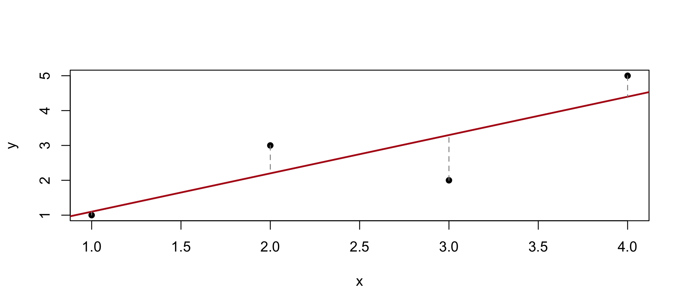
fit <- lm(y ~ x)

class(fit)

#> [1] "lm"

names(fit)          # a list underneath

#>  [1] "coefficients"  "residuals"     "effects"       "rank"         
#>  [5] "fitted.values" "assign"        "qr"            "df.residual"  
#>  [9] "xlevels"       "call"          "terms"         "model"

fit$coefficients

#>   (Intercept)             x 
#> -2.220446e-16  1.100000e+00

plot(x, y, pch = 16, xlab = "x", ylab = "y")
abline(fit, col = "#b31b1b", lwd = 2)
segments(x, y, x, fitted(fit), lty = 2, col = "grey55")   # the residuals

Four points scattered upward with the fitted least-squares line through them, and dashed vertical segments joining each point to the line to show its residual.

Combining list elements

pieces <- list(a = c(1, 2), b = c(3, 4), c = c(5, 6))

unlist(pieces)              # one flat vector, names kept

#> a1 a2 b1 b2 c1 c2 
#>  1  2  3  4  5  6

do.call(rbind, pieces)      # one matrix, one row per element

#>   [,1] [,2]
#> a    1    2
#> b    3    4
#> c    5    6

# 1. Build a diagonal matrix with the numbers 1 to 5 down the middle.
#
# 2. From m (the 2 x 3 matrix), pull the second column two ways: once
#    as a vector, once still a matrix.
#
# 3. l["readings"] and l[["readings"]]: which one can you take a mean of?
#    Find out with class(), not from memory.

diag(1:5)

#>      [,1] [,2] [,3] [,4] [,5]
#> [1,]    1    0    0    0    0
#> [2,]    0    2    0    0    0
#> [3,]    0    0    3    0    0
#> [4,]    0    0    0    4    0
#> [5,]    0    0    0    0    5

m[, 2]; m[, 2, drop = FALSE]

#> [1] 3 4

#>      [,1]
#> [1,]    3
#> [2,]    4

class(l["readings"]); class(l[["readings"]])   # list vs numeric

#> [1] "list"

#> [1] "numeric"

apply(): over rows and columns

You built these containers and picked things out of them. Now the other half: run one function over every row, column, group or file.

apply(temps, 1, mean)              # 1 = rows

#>  Compton   Reseda 
#> 15.33333 17.66667

apply(temps, 2, mean)              # 2 = columns

#>  Jan  Feb  Mar 
#> 13.0 16.0 20.5

rowMeans(temps); colMeans(temps)   # same answers, named and faster

#>  Compton   Reseda 
#> 15.33333 17.66667

#>  Jan  Feb  Mar 
#> 13.0 16.0 20.5

rowSums(temps)

#> Compton  Reseda 
#>      46      53

apply() with any function

apply(temps, 2, max)

#> Jan Feb Mar 
#>  14  17  22

apply(temps, 2, range)                       # two numbers per column

#>      Jan Feb Mar
#> [1,]  12  15  19
#> [2,]  14  17  22

apply(temps, 2, function(x) max(x) - min(x)) # write your own, inline

#> Jan Feb Mar 
#>   2   2   3

`split()`: one group per element

x <- c(12, 15, 19, 14, 17, 22)
g <- c("Compton", "Compton", "Compton", "Reseda", "Reseda", "Reseda")

split(x, g)

#> $Compton
#> [1] 12 15 19
#> 
#> $Reseda
#> [1] 14 17 22

`lapply()`: a list in, a list out

by_site <- split(x, g)

lapply(by_site, mean)

#> $Compton
#> [1] 15.33333
#> 
#> $Reseda
#> [1] 17.66667

`sapply()`: the same, simplified

sapply(by_site, mean)      # a named vector, not a list

#>  Compton   Reseda 
#> 15.33333 17.66667

sapply(by_site, length)

#> Compton  Reseda 
#>       3       3

sapply(by_site, range)     # two numbers each, so a matrix comes back

#>      Compton Reseda
#> [1,]      12     14
#> [2,]      19     22

apply(temps, 1, mean)      # same answers, from the matrix

#>  Compton   Reseda 
#> 15.33333 17.66667

Exercise 2

Exercise
Solution

# 1. One line: the highest reading in each city. One line: the highest
#    in each month.
#
# 2. One line: the range of each site in by_site. Why does that come
#    back as a matrix?

apply(temps, 1, max)   # margin 1 = rows = cities

#> Compton  Reseda 
#>      19      22

apply(temps, 2, max)   # margin 2 = columns = months

#> Jan Feb Mar 
#>  14  17  22

sapply(by_site, range)        # two numbers per site...

#>      Compton Reseda
#> [1,]      12     14
#> [2,]      19     22

dim(sapply(by_site, range))   # ...so sapply stacks them into a matrix

#> [1] 2 2

Reading a CSV

la <- read.csv("data/epa_pm25_la_county_2025.csv")
dim(la)

#> [1] 4757   22

# Uncomment and run once. Same file, fetched instead of clicked.
# dir.create("data", showWarnings = FALSE)
# download.file(paste0("https://arielortizbobea.github.io/aem6850/",
#                      "fall-2026/sessions/data/epa_pm25_la_county_2025.csv"),
#               "data/epa_pm25_la_county_2025.csv")

A data frame is a list of columns

is.list(la)             # a data frame IS a list

#> [1] TRUE

length(la)              # of 22 columns

#> [1] 22

head(sapply(la, class)) # so sapply walks the columns

#>                           Date                         Source 
#>                    "character"                    "character" 
#>                        Site.ID                            POC 
#>                      "integer"                      "integer" 
#> Daily.Mean.PM2.5.Concentration                          Units 
#>                      "numeric"                    "character"

Identifiers read as numbers

la$Site.ID[1]        # what R holds

#> [1] 60370016

colClasses: setting types at read time

la <- read.csv("data/epa_pm25_la_county_2025.csv",
               colClasses = c("Site.ID" = "character"))

la$Site.ID[1]

#> [1] "060370016"

unique(la$Site.ID)            # unique() drops repeats

#>  [1] "060370016" "060371103" "060371201" "060371302" "060371602" "060372005"
#>  [7] "060374008" "060374009" "060374010" "060376012" "060379035"

length(unique(la$Site.ID))    # ...so this counts monitors: eleven

#> [1] 11

Dates

la$Date[1]

#> [1] "01/01/2025"

class(la$Date)

#> [1] "character"

la$date <- as.Date(la$Date, format = "%m/%d/%Y")
class(la$date)

#> [1] "Date"

range(la$date)

#> [1] "2025-01-01" "2025-12-31"

Pulling pieces out of a date

d <- as.Date("2025-01-07")

c(month = format(d, "%m"), name = format(d, "%b"),
  year = format(d, "%Y"), doy = format(d, "%j"),
  day = weekdays(d))

#>     month      name      year       doy       day 
#>      "01"     "Jan"    "2025"     "007" "Tuesday"

la$month <- format(la$date, "%m")

%m/%d/%Y is a format string describing where the pieces are:

Dates are numbers

d + 30                                # thirty days later

#> [1] "2025-02-06"

as.Date("2025-03-01") - d             # how far apart

#> Time difference of 53 days

seq(d, by = "week", length.out = 4)   # a sequence of dates

#> [1] "2025-01-07" "2025-01-14" "2025-01-21" "2025-01-28"

seq(as.Date("2025-01-01"), as.Date("2025-12-01"), by = "month")

#>  [1] "2025-01-01" "2025-02-01" "2025-03-01" "2025-04-01" "2025-05-01"
#>  [6] "2025-06-01" "2025-07-01" "2025-08-01" "2025-09-01" "2025-10-01"
#> [11] "2025-11-01" "2025-12-01"

Checking for duplicate rows

Before averaging anything, find out what one row is.

key <- la[, c("Site.ID", "date")]

anyDuplicated(key)     # 0 means none; otherwise the first repeated row

#> [1] 695

sum(duplicated(key))   # how many rows repeat a site-day

#> [1] 1270

frm <- la[la$AQS.Parameter.Code == 88101 & la$POC == 1, ]

anyDuplicated(frm[, c("Site.ID", "date")])   # 0: one row per site-day now

#> [1] 0

More rows than site-days: something is duplicated, with no warning.
A site runs several instruments, each with a row on the same day.

tapply(): a matrix from two groupings

Numbers to summarise, what to group them by, a function to run on each group. Two groupings give one value per combination.

tb <- tapply(frm$Daily.Mean.PM2.5.Concentration,
             list(frm$Local.Site.Name, frm$month), mean)

dim(tb)

#> [1]  8 12

round(tb[, 1:6], 1)

#>                                  01   02  03   04   05   06
#> Compton                        21.3 13.4 8.7  5.8 15.5 10.8
#> Lancaster - Fairgrounds         4.1  1.8 2.6  4.9  6.0  6.1
#> Long Beach-Route 710 Near Road 18.4 11.4 8.7  9.0 10.2 11.2
#> Los Angeles-North Main Street  19.4 13.1 7.9 10.1 11.5 12.5
#> Pasadena                       25.4  9.6 7.7  9.1 10.3 11.9
#> Pico Rivera #2                 21.6 11.6 8.7  9.2 10.8 11.7
#> Reseda                         11.6  7.2 7.6  8.5  9.5 10.9
#> Signal Hill (LBSH)             20.6  7.9 4.7  8.1  9.0  9.3

reshape(): long and wide

tapply() gave a matrix. reshape() does the same turn on a data frame, and turns it back.

long <- data.frame(site  = c("A", "A", "B", "B"),
                   month = c("01", "02", "01", "02"),
                   pm25  = c(21.3, 13.4, 11.6, 7.2))
long

#>   site month pm25
#> 1    A    01 21.3
#> 2    A    02 13.4
#> 3    B    01 11.6
#> 4    B    02  7.2

wide <- reshape(long, direction = "wide",
                idvar = "site", timevar = "month", v.names = "pm25")
wide

#>   site pm25.01 pm25.02
#> 1    A    21.3    13.4
#> 3    B    11.6     7.2

reshape(): back to long

reshape(wide, direction = "long", idvar = "site",
        varying = list(2:3), v.names = "pm25", times = c("01", "02"))

#>      site time pm25
#> A.01    A   01 21.3
#> B.01    B   01 11.6
#> A.02    A   02 13.4
#> B.02    B   02  7.2

Long: one row per observation. Wide: one row per unit, one column per group.
idvar stays a row, timevar becomes columns, v.names is the value.

apply() over both margins

round(sort(apply(tb, 1, mean), decreasing = TRUE), 1)   # per site, all year

#>                        Compton  Los Angeles-North Main Street 
#>                           12.9                           12.7 
#>                 Pico Rivera #2 Long Beach-Route 710 Near Road 
#>                           12.3                           12.3 
#>                       Pasadena             Signal Hill (LBSH) 
#>                           11.4                           10.7 
#>                         Reseda        Lancaster - Fairgrounds 
#>                            9.2                            4.5

round(apply(tb, 2, mean), 1)                            # per month, all sites

#>   01   02   03   04   05   06   07   08   09   10   11   12 
#> 17.8  9.5  7.1  8.1 10.3 10.6  8.6 11.1  8.6  9.7 12.3 15.4

merge(): joining two tables

Results in one table, the thing you want to attach in another. merge() matches them on a shared column.

means  <- data.frame(site = rownames(tb), pm25 = round(apply(tb, 1, mean), 1))
coords <- unique(frm[, c("Local.Site.Name", "Site.Latitude", "Site.Longitude")])
names(coords) <- c("site", "lat", "lon")

nrow(means); nrow(coords)                    # count BEFORE

#> [1] 8

#> [1] 8

sites <- merge(means, coords, by = "site")
nrow(sites)                                  # and after

#> [1] 8

How merge() drops and duplicates rows

partial <- coords[coords$site != "Compton", ]   # pretend one site is missing

nrow(merge(means, partial, by = "site"))                # dropped

#> [1] 7

nrow(merge(means, partial, by = "site", all.x = TRUE))  # kept, with NA

#> [1] 8

Default keeps only keys in both tables: rows vanish, silently.
all.x = TRUE keeps the left table and fills with NA.
A duplicated key on the right multiplies rows instead.
Count rows before and after. Every time.

Reading many files

files <- list.files("data", pattern = "\\.csv$")
files

#> [1] "epa_pm25_compton_2025.csv"      "epa_pm25_la_county_2025.csv"   
#> [3] "la-weather-dec2024-feb2025.csv"

sapply(files, function(f) nrow(read.csv(file.path("data", f))))

#>      epa_pm25_compton_2025.csv    epa_pm25_la_county_2025.csv 
#>                            662                           4757 
#> la-weather-dec2024-feb2025.csv 
#>                             92

Writing files to disk

answers <- data.frame(site = rownames(tb),
                      mean = round(apply(tb, 1, mean), 1))

write.csv(answers, "results.csv", row.names = FALSE)   # text, anything reads it
saveRDS(answers, "results.rds")                        # R's own format
readRDS("results.rds")

Quick reference

Selected commands from today. The session page has all of them, grouped by topic.

Code	What it does
`matrix(x, nrow =, byrow =)` · `diag()`	Build one; the diagonal
`m[i, j]` · `m[, j, drop = FALSE]`	Index; keep it a matrix
`rbind()` · `cbind()`	Stack; widen
`l[["a"]]` vs `l["a"]`	The element vs a list of one
`unlist(l)` · `do.call(rbind, l)`	Flatten; stack
`apply(m, 1, f)` · `lapply()` · `sapply()`	A margin; a list; simplified
`split(x, g)` · `tapply(x, list(g1, g2), f)`	Groups; two groupings, one matrix
`as.Date(x, format =)` · `seq(d, by =)`	Text to date; a run of dates
`anyDuplicated(d)` · `unique(x)`	Any repeats; drop them
`merge(a, b, by =, all.x =)`	Join, keeping every row of `a`
`colClasses = c(id = "character")`	Protect identifiers at read time
`saveRDS()` · `readRDS()`	An R object, saved exactly as it was