AEM 6850

Empirical Methods for Applied Economists

Prof. Ariel Ortiz-Bobea

1 · Overview

Tuesday, August 25, 2026

Polls open

pollev.com/arielortizbobea090 · text arielortizbobea090 to 22333

A short background survey. Your answers shape how I teach the next few weeks. Graded quizzes and attendance will run on this same tool all semester.

Items 1–10 of the background survey run one at a time while people arrive. Item 11 (the free point) right after, as the graded-quiz demo. Say the calibration point out loud: the tool split and the AI answers decide how hard sessions 2–9 lean.

Objectives

By the end of this session you can:

• State what the course covers and navigate the course map.
• Run a script and find its outputs.
• Write down what a dataset should show, run the code, and check.
• Get your private course repository (repo) and commit a change in the browser.

About me

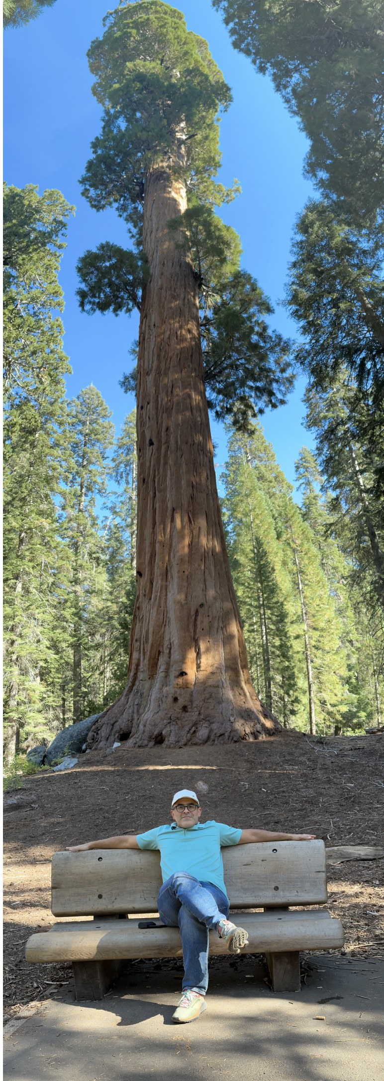
• Prof. Ariel Ortiz-Bobea: Dyson School and the Brooks School of Public Policy; at Cornell since 2014.
• Before Cornell: Resources for the Future; PhD, University of Maryland; Ministry of the Environment of the Dominican Republic.
• Research: how people cope with environmental change, especially how climate change affects the economy, and agriculture in particular. More at arielortizbobea.github.io.

Motivation

• Every empirical paper rests on data somebody found, cleaned, checked, and reshaped.
• Methods courses start after that work is done. This course teaches it.

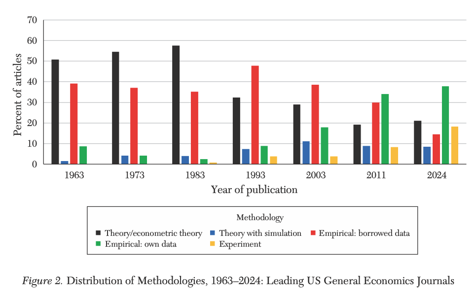
Economics is now an empirical field

Hamermesh (2025), update to “Six Decades of Top Economics Publishing” (JEL).

Green bars: papers built on data the authors assembled themselves, now the single largest category, 38% in 2024 vs 9% in 1963. That assembling is this course.

AI is arriving faster than the PC or the internet

Bick, Blandin & Deming (2024), “The Rapid Adoption of Generative AI”.

Blue dot: generative AI two years after launch, just under 40% adoption, about double the PC and the internet at the same age.

AI is changing research work

• It writes competent first drafts: code, summaries, extraction, text.
• This reduces the marginal cost of doing research.
• But increases the chances of making costly and yet potentially invisible mistakes.
• Key emerging skill: supervise and verify in robust and efficient ways.

Do not rush this slide. Everything downstream depends on students believing the last bullet. Ask the room: who has had a model hand them code that ran fine and was wrong?

AI models draft and execute code. You supervise and verify.

Error-free is not correct. A wrong number from code that runs clean is the key challenge of the AI era; this course builds the skills to catch it.

The course map

Twenty-eight meetings, two parts.

• Part I — foundations (1–12). Learn how to work with basic tabular data. Coding “by hand” through session 7. AI assistance enters in session 8.
• Part II — applications (13–28). We explore various families of unconventional data types and ways to acquire and process them.

Six families of data types

1. messy tables: clean real spreadsheets
2. text: from words into variables
3. documents: tables out of PDFs and scans
4. images: pixels into measurements
5. audio: speech, pauses, tone as data
6. maps & rasters: places, joins, exposures

Cross-cutting channels: downloads, APIs, scraping, vendors, archives, your own collection.

What we do not cover

• No causal inference, no econometric theory.
• No machine-learning theory: we use models, we do not derive them.
• No video, no network data (at least this year).

Why R?

• The habits transfer: acquire, clean, check, verify work the same in any language.
• R is free, open source, and built for data analysis. One install covers the course.
• Wide user base across fields, excellent graphics, answers easy to find.
• Python later is cheap; AI translation makes it cheaper. The habits carry.

The survey just showed the room’s tool split. Acknowledge Stata and Python users: nothing they know is wasted, and nothing here locks them in.

Install party

Do these in order: RStudio looks for R when it starts, so install R first.

1. Install R. cran.r-project.org → your operating system.

• macOS: there are two builds. Apple silicon (M1–M4) needs the arm64 installer; older Intel Macs need the x86_64 one. Apple menu → About This Mac tells you which you have.
• Windows: click “base”, then the download link. You do not need Rtools.

2. Install RStudio. posit.co/download/rstudio-desktop → the free Desktop version. It also bundles Quarto, a tool that turns scripts into reports (we use it later in the course). There is nothing else to install.

Check it worked

3. Open RStudio (not R) and type this into the Console, bottom left:

R.version.string

You should see version 4-point-something. If you see an error, or RStudio says it cannot find an R installation, raise your hand.

4. One setting, right now. Tools → Global Options → General: uncheck “Restore .RData into workspace at startup”, and set “Save workspace to .RData on exit” to Never.

Laptop refusing? posit.cloud is RStudio in a browser. Free, works today.

The four panes

• Console (bottom left): runs code the moment you press Return.
• Source (top left): scripts: code you keep.
• Environment (top right): the objects you have made.
• Plots / Files (bottom right): figures and your folder.

Today: type in the Console. Keep code worth keeping in Source.

Point at each pane on the projected RStudio while naming it. Land on: Console = scratch, Source = keep.

Onboarding: get your repo

• Everyone gets a private repository on GitHub: your course workspace.
• Every homework is handed in there. Nothing by email, nothing on Canvas.
• Today: account → repository → one commit. The pipeline works before any grade rides on it.

Everyone finishes this today, in the room. It runs entirely in a browser, so a half-installed laptop is no obstacle.

The three steps

1. Account. github.com/signup. Pick a username you would put on a CV.

2. Form. Your name · NetID · GitHub username. Scan, or open the Sign-up form link on Canvas:

3. Accept the invitation. We send the invitations in batches during class. Check email or github.com/notifications, then click Accept invitation.

Username = top-right menu on github.com, not the email. The form feeds the provisioning script: username in, repository + invitation out. While they type: export the CSV and run the sweep (runbook); re-run for stragglers.

Onboarding: your first commit

4. Edit the README in the browser. Click README.md, then the pencil icon. Fill in the three lines:

Name:
Program:
One dataset or question I would like to be able to handle by December:

5. Commit. Green “Commit changes…” button, top right. Type a short message (add my intro), leave “Commit directly to the main branch” selected, and click Commit changes.

6. Look at what you did. Reload the repository’s front page. Your text is there, and above it your message, add my intro, with a timestamp.

You just used version control

What just happened. You made a commit: a permanent, timestamped snapshot of your work. No git install, no terminal: the browser did it.

You will hand in the first few homeworks the same way: edit or drag files onto the repository page, then commit. Session 7 will explain what git did here.

7. Check in. The last poll of the day asks for your repository’s URL. Copy it from the address bar and paste it in. This is how we take attendance today, and it shows us your setup worked end to end.

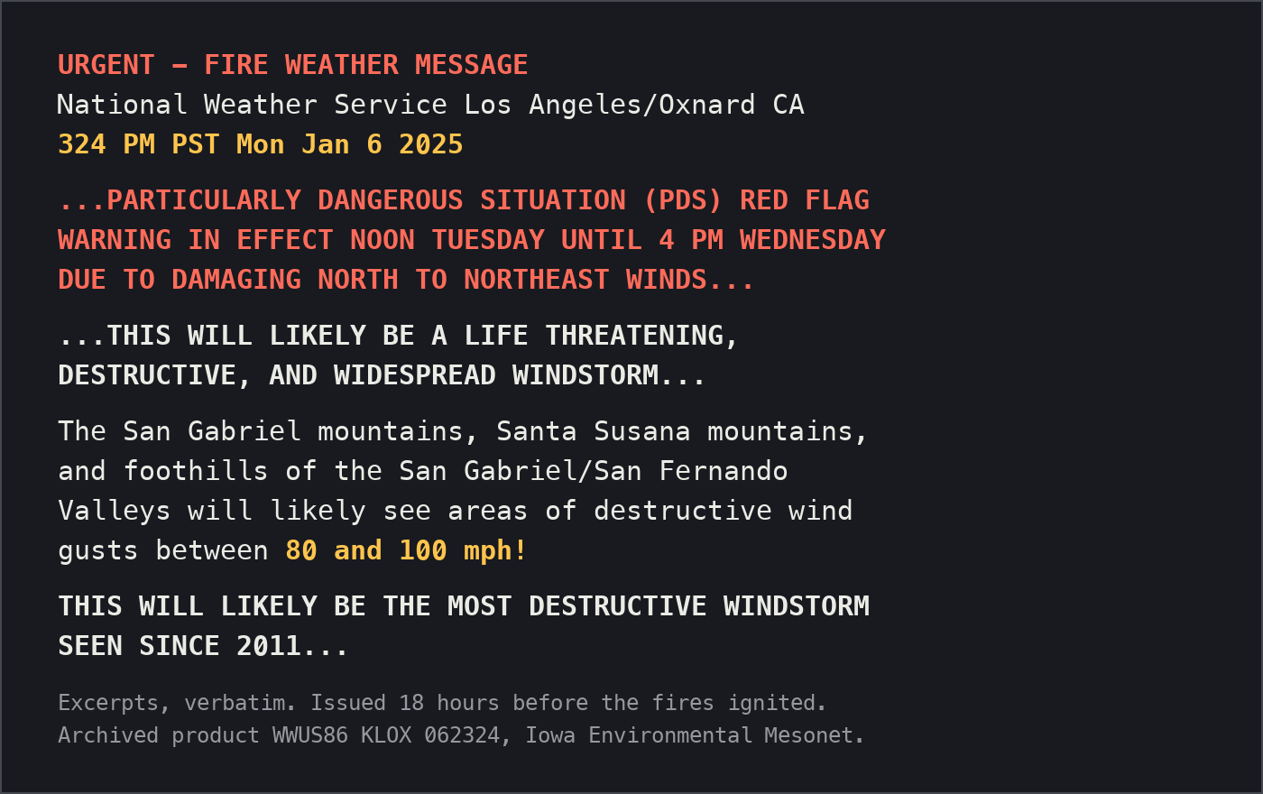
The warning, the day before

Read the amber lines out loud. This is the National Weather Service on January 6 at 3:24 PM, eighteen hours before ignition. It names the exact foothills where the Eaton fire exploded. This document is the “story” our data will be checked against.

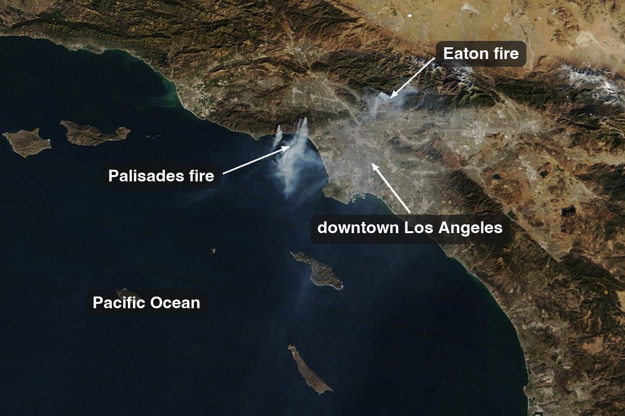
The January 2025 Los Angeles fires

Both ignited January 7, 2025 in Santa Ana winds near 100 mph, destroying about 16,000 structures. NASA Terra/MODIS.

Orient the room; many students are new to the US. Los Angeles sits on the Pacific coast. Palisades fire by the ocean, Eaton fire inland above Altadena, the grey between them is the city. This event runs through every homework this semester.

What should the data show?

The story so far, from the previous slides: both fires exploded on January 7, driven by a violent windstorm, in the middle of a drought. Strong wind spreads fire; dry ground feeds it.

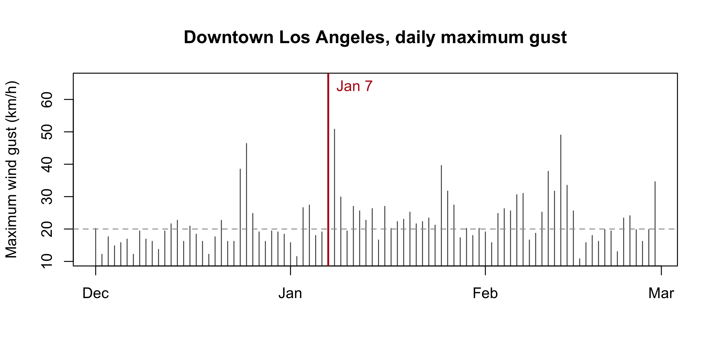
We are about to plot the strongest daily wind gust in downtown Los Angeles, December 2024 through February 2025.

First write down what the data should show if the story is right. Turn each into a number or a date.

1. Which date should show the biggest gust?
2. A typical winter day gusts near 20 km/h. How tall should the spike be?
3. What was December’s total rainfall, in millimetres?

Say it plainly: the story makes promises about the data. Jan 7 should be the spike (Q1). The spike’s height is genuinely open; the anchor is 20 (Q2, answer 66). Drought should mean near-zero December rain (Q3, answer 0.5 mm). If the plot breaks a promise, something is wrong with the data, the code, or the story.

Step 1: Pull the data

The data comes from Open-Meteo, which serves historical weather as a plain CSV over a URL. No account, no key, no package.

url <- paste0(
  "https://archive-api.open-meteo.com/v1/archive",
  "?latitude=34.05&longitude=-118.24",
  "&start_date=2024-12-01&end_date=2025-02-28",
  "&daily=wind_gusts_10m_max,wind_speed_10m_max,",
  "temperature_2m_max,relative_humidity_2m_min,precipitation_sum",
  "&timezone=America%2FLos_Angeles&format=csv"
)

la <- read.csv(url, skip = 3)
names(la) <- c("date", "gust", "wind", "tmax", "rh_min", "precip")
la$date <- as.Date(la$date)

Step 2: Look at what arrived

Never compute on a file you have not looked at. Three lines, every time:

dim(la)

#> [1] 90  6

str(la)

#> 'data.frame':    90 obs. of  6 variables:
#>  $ date  : Date, format: "2024-12-01" "2024-12-02" ...
#>  $ gust  : num  20.2 12.2 17.6 14.8 15.8 16.9 12.2 19.4 16.9 16.2 ...
#>  $ wind  : num  7.5 3.8 6.3 4 5 5 4.9 8 6.3 6.6 ...
#>  $ tmax  : num  24.5 22.6 21.5 19.7 21.2 25 26.3 21.2 19.7 20.2 ...
#>  $ rh_min: int  12 19 36 52 28 14 10 27 27 6 ...
#>  $ precip: num  0 0 0 0 0 0 0 0 0 0 ...

summary(la$gust)

#>    Min. 1st Qu.  Median    Mean 3rd Qu.    Max. 
#>   10.80   16.90   20.00   22.71   25.60   65.90

Step 3: One plot

plot(la$date, la$gust,
     type = "h", col = "grey30",
     xlab = "", ylab = "Maximum wind gust (km/h)",
     main = "Downtown Los Angeles, daily maximum gust")

abline(h = median(la$gust), lty = 2, col = "grey60")
abline(v = as.Date("2025-01-07"), col = "#b31b1b", lwd = 2)
text(as.Date("2025-01-07"), max(la$gust), "  Jan 7",
     col = "#b31b1b", adj = c(0, 1))

Step 4: Reconcile

Now compare the screen against what you wrote down.

la$date[which.max(la$gust)]                 # 1. the windiest day

#> [1] "2025-01-07"

max(la$gust) / median(la$gust)              # 2. how unusual it was

#> [1] 3.295

sum(la$precip[format(la$date, "%Y-%m") == "2024-12"])  # 3. December rain, in mm

#> [1] 0.5

• The windiest day of the winter is the day the fires started.
• It was 3.3× a normal day.
• December’s total rainfall: half a millimetre.

Quick reference

On the session page: the install checklist, every command from today, and the links.

:::