HW1 solution · How bad was the air?
This page is the instructor’s solution to HW1. Two R scripts and a master file download EPA’s raw file, clean it, and draw the target figure below. Run from a fresh clone, they write the same PNG that is posted here. The page walks through the approach and the code and lists where submissions went wrong. It then explains a mistake in the target as first posted and ends with the three scripts in full.
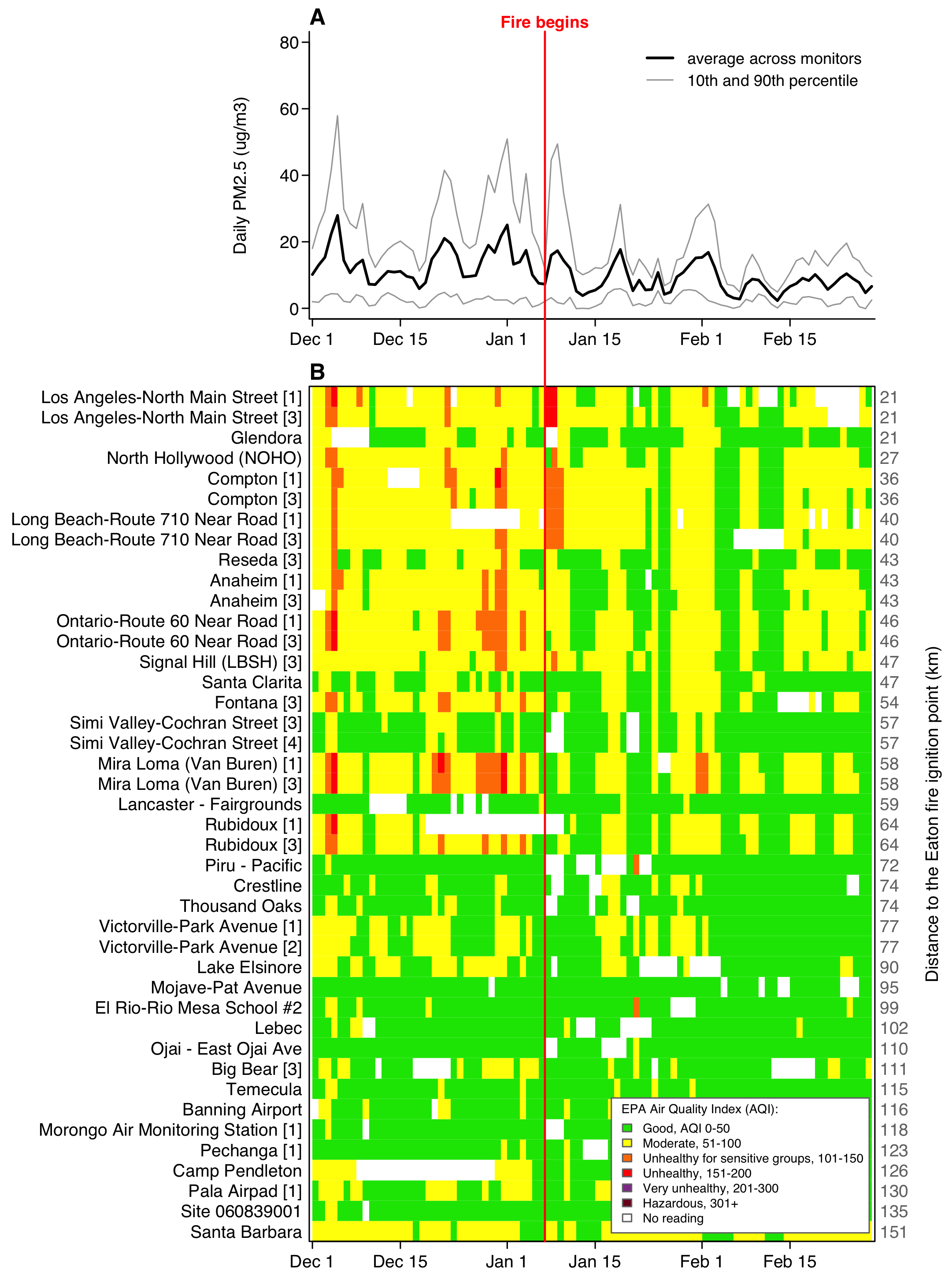
From download to figure
The work runs in seven steps.
- Download the CSV into
data/. Later runs find the file there and skip the download. - Read it with
Site.IDkept as text, keep the 90 days from 1 December to 28 February, and check that the instrument key is unique on each day. - Measure each instrument’s distance from the Eaton Fire’s ignition point and sort the instruments nearest first. Give each one a row label.
- Build two matrices with one row per instrument and one column per day, one of PM2.5 and one of AQI, and drop the instruments that reported on fewer than 60 days.
- Save everything the figure needs as one list in
data_clean/hw1_clean.rds. - Read that list back, compute the network’s daily mean and percentiles, and put each AQI value in one of EPA’s six categories.
- Draw both panels into one PNG,
figures/hw1_target.png.
code/1_get_clean_data.R does steps 1 to 5, and code/2_plot_figure.R does steps 6 and 7. The master file, code/run_everything.R, sources the two in order.
Downloading and cleaning happen once, and the figure gets redrawn dozens of times while you adjust margins, labels and the key. With the cleaning in its own script, each redraw runs script 2 alone, in seconds, with no download. The .rds file is the only link between the scripts. Script 2 reads all its data from that file, so it draws the same figure whether script 1 ran a minute ago or last week. A change to the drawing code cannot alter the data.
How the code is organised
hw1/
  hw1.Rproj                 open this first
  code/
    run_everything.R        master file: two source() calls
    1_get_clean_data.R      download, clean, save
    2_plot_figure.R         read, summarise, draw
  data/                     the CSV, exactly as downloaded
  data_clean/               hw1_clean.rds
  figures/                  hw1_target.png
hw1.Rproj sits at the project root. Opening it sets the working directory to hw1/, so every path in the code starts from there: "data/...", "figures/...". Raw data stays in data/, and anything the code computed goes to data_clean/.
The parameter block. Each script opens with a list called misc. Script 1’s block has the download URL, the file paths, the start and end dates, the 60-day minimum, the fire’s coordinates and the two km-per-degree constants. The block in script 2 has the file paths, the ignition date, the AQI category bounds, the six colours and their labels, the colour for no reading, and the figure’s size, point size, margins and text size. Each of these values is typed once, at the top, so a change to one of them happens on one line. Script 2 takes the window’s start and end from the .rds file, so the window is set in script 1 only. A few drawing values stay in the body of script 2: the tick dates at lines 87–88, panel A’s upper limit of 80 at lines 105 and 117, and the 2.6 in the panel heights at lines 98 and 173. The 80 and the 2.6 are each typed twice, and the two copies must change together.
The sections. Comment lines ending in ---- divide each script, and RStudio lists them in the document outline. Script 1 has three: Preliminary (parameters and folders), Get the data, and Clean, which ends by saving the list and printing a short report. In script 2 the three are Preliminary (parameters, the figures folder, reading the .rds, and the one small function), Compute daily summaries, and Create the figure. The last one has a sub-section for each panel, also marked with dashes. Each panel’s code sits in its own if (T) { } block, which lets you fold it away or run it as one piece.
Running it. From a fresh clone, open hw1.Rproj and run
source("code/run_everything.R")or, from a terminal in hw1/, Rscript code/run_everything.R. The master file empties the workspace first, so a script that uses an object no line creates stops with an error. Script 1 creates data/ and data_clean/ and downloads the file if it is missing, and script 2 creates figures/. The code uses base R only, so there is nothing to install. On a fresh clone, script 1 prints:
42 monitors at 33 sites, reporting 60+ of the 90 days
3555 of 3780 cells have a reading (94%)
nearest 21 km, farthest 151 km from the Eaton fire
Saved: data_clean/hw1_clean.rds
The code, step by step
Each excerpt is copied from the scripts, with the file name and line numbers.
Reading the file
read.csv() guesses a type for each column. It reads Site.ID as a number, and 060371103 becomes 60371103 with no warning. colClasses keeps that one column as text from the start.
code/1_get_clean_data.R, line 56
d <- read.csv(misc$file, colClasses = c("Site.ID" = "character"))The window and the instrument key
The file writes dates as month/day/year text, so as.Date() needs the format spelled out. One logical index then keeps the 90 days. The key pastes site, POC and parameter code together, and stopifnot() halts the script if any instrument appears twice on the same day.
code/1_get_clean_data.R, lines 69–77
  d$date <- as.Date(d$Date, format = "%m/%d/%Y")
  d <- d[d$date >= misc$start & d$date <= misc$end, ]

  # A site is a place; a monitor is one instrument at that place, and a busy
  # site runs several. Site plus POC plus parameter names the instrument.
  # That key is unique on any given day, so every instrument can have its own
  # row in the heat map and nothing is counted twice.
  d$monitor <- paste(d$Site.ID, d$POC, d$AQS.Parameter.Code)
  stopifnot(anyDuplicated(paste(d$monitor, d$date)) == 0)
Distance from the fire and the row order
Each difference in degrees becomes kilometres through its constant, and Pythagoras gives the distance. duplicated() keeps one row per instrument, and order() sorts those rows nearest first. That sort fixes the order of panel B, so the code never names a site.
code/1_get_clean_data.R, lines 82–88
  north <- (d$Site.Latitude  - misc$fire_lat) * misc$km_lat
  east  <- (d$Site.Longitude - misc$fire_lon) * misc$km_lon
  d$km  <- sqrt(north^2 + east^2)

  # One row per monitor, nearest the fire first.
  m <- d[!duplicated(d$monitor), ]
  m <- m[order(m$km), ]
The monitor-by-day grid and the 60-day rule
tapply() builds a matrix with one row per instrument and one column per day. The factor’s levels list all 90 dates, so every day gets a column even if no instrument reported on it. The key allows one reading per instrument per day, so mean returns that reading unchanged. Indexing with [m$monitor, ] puts the rows in distance order. A day an instrument missed stays NA.
code/1_get_clean_data.R, lines 102–105
  cal     <- seq(misc$start, misc$end, by = "day")
  day     <- factor(format(d$date), levels = format(cal))
  grid_pm  <- tapply(d$pm25, list(d$monitor, day), mean)[m$monitor, ]
  grid_aqi <- tapply(d$aqi,  list(d$monitor, day), mean)[m$monitor, ]
The 60-day rule counts the readings in each row and keeps the rows with at least misc$min_days. One logical vector subsets both grids and the monitor table, so the three stay aligned.
code/1_get_clean_data.R, lines 110–113
  enough   <- apply(!is.na(grid_pm), 1, sum) >= misc$min_days
  grid_pm  <- grid_pm[enough, ]
  grid_aqi <- grid_aqi[enough, ]
  m        <- m[enough, ]
Row labels with POC brackets
Each label starts as the site name. The one site with a blank name gets its ID. Where a site has more than one instrument, the POC goes in brackets after the name. This test runs before the 60-day rule, so seven rows in the target keep a bracket although their site’s other instruments were dropped. Reseda’s [3] is the first of them.
code/1_get_clean_data.R, lines 94–98
  m$label <- m$site
  blank <- m$label == ""
  m$label[blank] <- paste("Site", m$Site.ID[blank])
  many <- m$site %in% m$site[duplicated(m$site)]
  m$label[many] <- paste0(m$site[many], " [", m$POC[many], "]")
Panel A’s daily mean and percentiles
pctl() sorts a day’s readings, which also drops the NAs, and picks one value by position. With 40 readings on a day, the 10th percentile is the 4th smallest and the 90th is the 36th.
code/2_plot_figure.R, lines 67–71
  pctl <- function(x, p) {
    x <- sort(x)
    if (length(x) == 0) return(NA)
    x[max(1, round(p * length(x)))]
  }
apply() with 2 runs down each column of the PM2.5 grid, one day at a time. Panel A then draws the two percentiles in grey and the mean in black with lines(), at lines 111–113.
code/2_plot_figure.R, lines 77–79
  avg <- apply(d$grid_pm, 2, mean, na.rm = TRUE)
  p10 <- apply(d$grid_pm, 2, pctl, p = 0.10)
  p90 <- apply(d$grid_pm, 2, pctl, p = 0.90)
Panel B’s colours
findInterval() turns each AQI value into its category number, 1 to 6, using the category lower bounds c(0, 51, 101, 151, 201, 301) from the parameter block. band[] <- keeps the matrix shape and fills it with those numbers.
code/2_plot_figure.R, lines 83–84
  band   <- d$grid_aqi
  band[] <- findInterval(d$grid_aqi, misc$breaks)
image() then gives each number a colour. Left alone, it spreads the six colours over the range of the data. Nothing in this window goes past category 4, so the six colours would stretch over categories 1 to 4, and categories 3 and 4 would come out in colours 4 and 6. A zlim running from 0.5 to 6.5 pins the range to all six categories, and category k gets colour k whatever the data contain. The matrix goes in upside down, band[nrows:1, ], because image() draws row 1 at the bottom, and t() turns it so the days run along the x axis. Cells with no reading are NA. image() leaves them undrawn, and the white background of the PNG shows through. The assignment’s tip paints the panel white with rect() before image(), which gives the same result. Line 144 of code/2_plot_figure.R keeps that call commented out because the PNG already starts white. The comment above it mentions grey because an earlier version painted missing days grey. The dates go in as plain numbers for the reason given further down.
code/2_plot_figure.R, lines 150–151
    image(x = as.numeric(d$cal), y = 1:nrows, z = t(band[nrows:1, ]), add = TRUE,
          col = misc$cols, zlim = c(0.5, length(misc$cols) + 0.5))
One date axis for both panels
The red line runs straight through both panels only if their x axes match exactly. Both panels use the same margins, set once in the parameter block.
code/2_plot_figure.R, lines 53–54
  misc$mar    <- c(2.0, 15.4, 1.4, 3.7)   # shared, so the two x axes line up;
                                          # left fits the longest site name exactly
The two plot() calls share an xlim that runs half a day either side of the window, because each heat-map cell is one day wide and centred on its date. xaxs = "i" stops plot() from adding 4 percent of padding at each end. Panel A’s call at lines 109–110 uses the same xlim and xaxs.
code/2_plot_figure.R, lines 140–141
    plot(NA, xlim = c(d$start - 0.5, d$end + 0.5), ylim = c(0.5, nrows + 0.5),
       axes = FALSE, xlab = "", ylab = "", xaxs = "i", yaxs = "i")
The red line
The line is drawn once, from panel B. It starts at the bottom of B and runs up through the gap to the top of panel A, and xpd = NA lets it leave the plot region. The top end comes from the panel sizes: par("pin") is B’s plot region in inches, par("mai") its margins, and the layout heights make panel A’s figure 1/2.6 the height of B’s. Panel A carries the red “Fire begins” label at the same date, at line 122.
code/2_plot_figure.R, lines 171–176
    per_in   <- nrows / par("pin")[2]                        # B's y units per inch
    fig_b_in <- par("pin")[2] + par("mai")[1] + par("mai")[3] # B's figure height
    fig_a_in <- fig_b_in / 2.6                                # from layout heights
    a_plot   <- fig_a_in - par("mai")[1] - par("mai")[3]      # A's plot height
    y_top    <- nrows + 0.5 + per_in * (par("mai")[3] + par("mai")[1] + a_plot)
    lines(c(misc$ignite, misc$ignite), c(0.5, y_top), col = "red", lwd = 1.5, xpd = NA)
The key
One legend() call draws the key in panel B’s lower right corner. fill gives each label a coloured box. The labels and colours come from the parameter block, which holds all six categories, so the key lists each one whether or not it occurs. “No reading” and white are added at the end.
code/2_plot_figure.R, lines 160–164
      legend("bottomright", inset = 0.01, bg = "white", box.col = "grey45",
           cex = misc$cex * 0.72, y.intersp = 1,
           title = "EPA Air Quality Index (AQI):", title.adj = 0.1,
           legend = c(misc$labs, "No reading"),
           fill   = c(misc$cols, misc$no_data), border = "grey45")
The figure size
png() takes inches here, so the parameter block divides 183 and 247 mm by 25.4. The same call sets the resolution to the 300 dpi the assignment asks for. It also sets the point size, the base text size that every cex in the code scales.
code/2_plot_figure.R, lines 50–52
  misc$width  <- 183 / 25.4                # 7.20 in
  misc$height <- 247 / 25.4                # 9.72 in
  misc$pt     <- 9
code/2_plot_figure.R, lines 96–97
  png(misc$fig, width = misc$width, height = misc$height,
      units = "in", res = 300, pointsize = misc$pt)
Where submissions went wrong
Of the 39 students enrolled, 38 submitted. Each project was run from a fresh clone. Twenty-eight ran with no change to the code, some after their uploaded files were moved into the right folders, which cost nothing. Two more ran once their output folders were created, and eight needed a fix to the code before they ran. Of the 38 figures, 21 matched the target on every item the graders checked. The three lists below follow the rubric’s three dimensions, Replicability, Similarity and Coding, in that order. The counts are numbers of submissions, and some had more than one problem.
Running on a fresh machine
- No download step, or the download commented out (3). Put
download.file()in script 1, behindfile.exists(), so a fresh clone fetches the file itself. - A broken or empty download URL (2). Copy the URL from the assignment page into the parameter block and test it from a fresh clone.
- An object that existed only in the R session (2). No line of the scripts creates it, so the code ran only in the session where it was made. Restart R and source
run_everything.Rbefore you submit. - Output folders never created (4). Call
dir.create("figures", showWarnings = FALSE)before the first file is written there, and the same fordata/anddata_clean/. install.packages()inside a script (1). Delete it. This figure needs base R only.- An empty
run_everything.R(1). It needs twosource()calls, in order. - The figure written to the wrong path (1). Write
figures/hw1_target.png, with the path in the parameter block. - Reading an
.rdsfile uploaded to the repo (1) in place of the one script 1 writes. Read the path script 1 saves to, and leavedata_clean/out of the upload.
The figure
- Panels A and B on different date axes (7). Different left or right margins shift one panel, and the 7 January line breaks between them. Give both panels the same
mar, the samexlimandxaxs = "i". - Category colours shifted (4).
image()got six colours with nobreaksorzlim, so orange cells came out red and red cells maroon. Addzlim = c(0.5, 6.5). - Row labels missing, or numbers in place of site names (4). Write the labels with
mtext()on side 2, as at lines 179–180 ofcode/2_plot_figure.R. - Instruments merged into one row per site (3), giving 33 or 40 rows where the target has 42. Build the key from all three columns,
Site ID,POCandAQS Parameter Code. - Red line missing from panel B (2). Draw it from panel B with
xpd = NA, as above. - Wrong figure size (2). Use
width = 183 / 25.4andheight = 247 / 25.4withunits = "in". - Panel A missing from the saved file (1). The PNG got two pages, and a PNG file keeps only the last one. Call
layout()once, before the firstplot(), so the twoplot()calls fill its two slots on one page. - POC brackets lost to a typo (1). Without its hyphen, the arrow
<-becomes the comparison<. R evaluates the comparison and discards the result without an error. Put the hyphen back.
Three more differences were common and cost no points.
- Panel A keeps the 4 percent padding
plot()adds at each end (10), so its lines stop short of the grid’s edges.xaxs = "i"removes it. - Distance labels one kilometre off (many). The assignment page gave about 111 and 92 km per degree and said the target used 111.32 and 92.10. A one-kilometre difference cost nothing.
- Percentiles from
quantile()(several). It interpolates between readings, so its grey lines differ slightly fromsort()and an index.
The code
- Values typed into the code that belong in the parameter block, three or more of them (16). The file names, the window and ignition dates, the fire’s coordinates, the km-per-degree constants and the six AQI colours go in
miscat the top, as the assignment page asks, and the code refers to them asmisc$.... - A script with no comments on its working steps (7). Add one comment per step that says what it does and why.
run_everything.Rholding copies of the scripts (2). Twosource()calls keep each line of code in one file.
A mistake in the target
The target as first posted had a flaw of its own. Panel B was drawn with image(x = d$cal, ...), where d$cal holds Dates. image() puts each cell’s edges halfway between neighbouring x values, and it finds that half with 0.5 * diff(x). For Dates, diff() returns a time difference. R rounds a time difference to whole days before it adds it to a Date or subtracts it from one, and half a day rounds to 0. The edges landed on the dates themselves, which gave the cell for 1 December zero width and put each of the other 89 days half a day to the left of its date. A plain number such as the 0.5 in d$start - 0.5 keeps its half day, so the xlim above is unaffected. You can see the difference in any R session:
Console, any R session
x <- as.Date(c("2024-12-01", "2024-12-02"))
x[1] - 0.5 * diff(x)     # "2024-12-01": the half day rounds to zero
as.numeric(x)[1] - 0.5   # 20057.5, half a day before 1 December
unclass(x[1] - 0.5)      # 20057.5: a plain 0.5 keeps the half day
Three graders spotted it. The target was corrected and re-posted before grades went out, and no student lost points over it. The fix passes the dates to image() as plain numbers, which keep their half days.
code/2_plot_figure.R, lines 148–151
    # x as plain numbers: given Dates, image() rounds the half-day cell edges
    # to whole days, which drops 1 December and shifts every day half a day left.
    image(x = as.numeric(d$cal), y = 1:nrows, z = t(band[nrows:1, ]), add = TRUE,
          col = misc$cols, zlim = c(0.5, length(misc$cols) + 0.5))
The full code
These are the three files exactly as they run.
code/run_everything.R
# =============================================================
# AEM 6850 - HW1: "How bad was the air?"
# Master file. Runs the whole thing, in order.
#
# Open hw1.Rproj first. It sits at the project root, so the working
# directory is hw1/ and every path below is relative to it.
#
#   source("code/run_everything.R")     from the R console
#   Rscript code/run_everything.R       from a terminal, run in hw1/
#
# 1_get_clean_data.R  downloads the EPA files, writes data_clean/hw1_clean.rds
# 2_plot_figure.R     reads that, writes figures/hw1_target.png
# =============================================================

  rm(list = ls())

  source("code/1_get_clean_data.R")
  source("code/2_plot_figure.R")
code/1_get_clean_data.R
# =============================================================
# AEM 6850 - HW1: "How bad was the air?"
# Script 1 of 2 - get the data and clean it.
#
# Downloads one CSV of EPA daily PM2.5 for the monitors around the January
# 2025 Los Angeles fires, keeps the 90-day window, and puts the monitors in
# order of how far they sit from the fire. Writes one object for the
# plotting script.
#
# Writes: data_clean/hw1_clean.rds
#
# Open hw1.Rproj first. It sits at the project root, so the working
# directory is hw1/ and every path below is relative to it.
#
#   source("code/1_get_clean_data.R")
# =============================================================


# 1). Preliminary ----

  # Packages: none. Base R only.

  # Parameters
  misc <- list()
  misc$url      <- "https://arielortizbobea.github.io/assets/data/epa_pm25_la_fires_2024_2025.csv"
  misc$file     <- "data/epa_pm25_la_fires_2024_2025.csv"
  misc$clean    <- "data_clean/hw1_clean.rds"
  misc$start    <- as.Date("2024-12-01")
  misc$end      <- as.Date("2025-02-28")
  misc$min_days <- 60                  # of the 90; drop instruments that rarely report

  # Where the Eaton fire started, from CAL FIRE's own incident record.
  # The Palisades fire started the same week, 40 km west, but its smoke blew
  # straight out to sea; Eaton is the one whose plume crossed the monitored
  # basin, so distances here are measured from Eaton.
  misc$fire_lat <- 34.203483
  misc$fire_lon <- -118.069155

  # Turning a difference in degrees into a distance in kilometres. A degree
  # of latitude is about 111 km anywhere on Earth. A degree of longitude is
  # shorter, and shorter still the further you are from the equator: at Los
  # Angeles it is about 92 km.
  misc$km_lat <- 111.32
  misc$km_lon <- 92.10

  dir.create("data",       showWarnings = FALSE)
  dir.create("data_clean", showWarnings = FALSE)


# 2). Get the data ----

  # One file, one line. It is a plain CSV on the web, so download.file()
  # fetches it and read.csv() opens it exactly like a local file.
  if (!file.exists(misc$file)) download.file(misc$url, misc$file)

  d <- read.csv(misc$file, colClasses = c("Site.ID" = "character"))

  # Site.ID is a LABEL, not a quantity. Left to itself read.csv() calls the
  # column an integer and the leading zero disappears: 060371103 becomes
  # 60371103, silently. colClasses protects it at read time.


# 3). Clean ----

  names(d)[names(d) == "Daily.Mean.PM2.5.Concentration"] <- "pm25"
  names(d)[names(d) == "Local.Site.Name"]                <- "site"
  names(d)[names(d) == "Daily.AQI.Value"]                <- "aqi"

  d$date <- as.Date(d$Date, format = "%m/%d/%Y")
  d <- d[d$date >= misc$start & d$date <= misc$end, ]

  # A site is a place; a monitor is one instrument at that place, and a busy
  # site runs several. Site plus POC plus parameter names the instrument.
  # That key is unique on any given day, so every instrument can have its own
  # row in the heat map and nothing is counted twice.
  d$monitor <- paste(d$Site.ID, d$POC, d$AQS.Parameter.Code)
  stopifnot(anyDuplicated(paste(d$monitor, d$date)) == 0)

  # How far each monitor sits from the fire. The coordinates come with the
  # file, so no site is named anywhere in this script: the distance decides
  # the order the monitors appear in.
  north <- (d$Site.Latitude  - misc$fire_lat) * misc$km_lat
  east  <- (d$Site.Longitude - misc$fire_lon) * misc$km_lon
  d$km  <- sqrt(north^2 + east^2)

  # One row per monitor, nearest the fire first.
  m <- d[!duplicated(d$monitor), ]
  m <- m[order(m$km), ]

  # Label with the site name, and add the POC only where a site runs more
  # than one instrument, so those rows stay distinguishable. One site in
  # the file, 060839001 in Santa Barbara County, ships with a blank name;
  # it gets its ID instead, so no row is left unlabelled.
  m$label <- m$site
  blank <- m$label == ""
  m$label[blank] <- paste("Site", m$Site.ID[blank])
  many <- m$site %in% m$site[duplicated(m$site)]
  m$label[many] <- paste0(m$site[many], " [", m$POC[many], "]")

  # One column per calendar day. Days a monitor did not report stay NA,
  # which is what makes the gaps visible in the figure.
  cal     <- seq(misc$start, misc$end, by = "day")
  day     <- factor(format(d$date), levels = format(cal))
  grid_pm  <- tapply(d$pm25, list(d$monitor, day), mean)[m$monitor, ]
  grid_aqi <- tapply(d$aqi,  list(d$monitor, day), mean)[m$monitor, ]

  # Some instruments sample one day in three, or one in six. Their rows are
  # mostly gaps, and a wall of grey hides the pattern in the rows that do
  # report every day, so keep only the instruments that report often enough.
  enough   <- apply(!is.na(grid_pm), 1, sum) >= misc$min_days
  grid_pm  <- grid_pm[enough, ]
  grid_aqi <- grid_aqi[enough, ]
  m        <- m[enough, ]

  saveRDS(list(grid_pm  = grid_pm,   # monitor x day, concentrations
               grid_aqi = grid_aqi,  # monitor x day, EPA's own AQI value
               label   = m$label,   # row labels, nearest the fire first
               km      = m$km,      # km from the Eaton fire
               cal     = cal,
               start   = misc$start,
               end     = misc$end),
          misc$clean)

  cat(sprintf("%d monitors at %d sites, reporting %d+ of the 90 days\n",
              nrow(m), length(unique(m$site)), misc$min_days))
  cat(sprintf("%d of %d cells have a reading (%d%%)\n",
              sum(!is.na(grid_pm)), length(grid_pm),
              round(100 * sum(!is.na(grid_pm)) / length(grid_pm))))
  cat(sprintf("nearest %.0f km, farthest %.0f km from the Eaton fire\n",
              min(m$km), max(m$km)))
  cat("Saved:", misc$clean, "\n")

# the end
code/2_plot_figure.R
# =============================================================
# AEM 6850 - HW1: "How bad was the air?"
# Script 2 of 2 - the target figure.
#
# Reads data_clean/hw1_clean.rds, written by 1_get_clean_data.R, and
# produces: figures/hw1_target.png
#
#   A  the network as a whole: the daily average across monitors, with the
#      10th and 90th percentile of monitors on the same day
#   B  every monitor, every day, coloured by EPA's daily AQI category,
#      ordered by distance from the fire
#
# Open hw1.Rproj first. It sits at the project root, so the working
# directory is hw1/ and every path below is relative to it.
#
#   source("code/2_plot_figure.R")
# =============================================================


# 1). Preliminary ----

  # Packages: none. Base R only.

  # Parameters
  misc <- list()
  misc$clean    <- "data_clean/hw1_clean.rds"
  misc$fig      <- "figures/hw1_target.png"
  misc$ignite   <- as.Date("2025-01-07")

  # Color is EPA's Air Quality Index: six categories, six published colors,
  # nothing else. Breaks are the category lower bounds; findInterval() puts
  # each day's AQI into its band.
  misc$breaks <- c(0, 51, 101, 151, 201, 301)
  misc$cols   <- c("#00E400",    # Good
                   "#FFFF00",    # Moderate
                   "#FF7E00",    # Unhealthy for sensitive groups
                   "#FF0000",    # Unhealthy
                   "#8F3F97",    # Very unhealthy
                   "#7E0023")    # Hazardous
  misc$labs   <- c("Good, AQI 0-50",
                   "Moderate, 51-100",
                   "Unhealthy for sensitive groups, 101-150",
                   "Unhealthy, 151-200",
                   "Very unhealthy, 201-300",
                   "Hazardous, 301+")
  misc$no_data <- "white"

  # Figure size and text. One place to change any of it. 183 x 247 mm is a
  # full-page, double-column figure in some journals
  misc$width  <- 183 / 25.4                # 7.20 in
  misc$height <- 247 / 25.4                # 9.72 in
  misc$pt     <- 9
  misc$mar    <- c(2.0, 15.4, 1.4, 3.7)   # shared, so the two x axes line up;
                                          # left fits the longest site name exactly
  misc$cex    <- 1.05                     # one size for every axis label

# Create folder for figure
  dir.create("figures", showWarnings = FALSE)

# Read data
  d <- readRDS(misc$clean)

# Small function
# The 10th and 90th percentile of a day's readings. sort() drops the
# monitors that did not report, then one value is picked by position, so
# this needs nothing beyond sorting and indexing.
  pctl <- function(x, p) {
    x <- sort(x)
    if (length(x) == 0) return(NA)
    x[max(1, round(p * length(x)))]
  }


# 2). Compute daily summaries ----

  # Compute summaries
  avg <- apply(d$grid_pm, 2, mean, na.rm = TRUE)
  p10 <- apply(d$grid_pm, 2, pctl, p = 0.10)
  p90 <- apply(d$grid_pm, 2, pctl, p = 0.90)

  # Which color bin every cell falls in. findInterval() turns a number into
  # the position of the band it falls in. NA stays NA.
  band   <- d$grid_aqi
  band[] <- findInterval(d$grid_aqi, misc$breaks)

  # Tick marks on the 1st and 15th of each month, labelled "Dec 1", "Dec 15"...
  ticks <- as.Date(c("2024-12-01", "2024-12-15", "2025-01-01",
                     "2025-01-15", "2025-02-01", "2025-02-15"))
  tlabs <- paste(format(ticks, "%b"), as.numeric(format(ticks, "%d")))
  nrows  <- nrow(d$grid_pm)


# 3). Create the figure ----

  # Header
  png(misc$fig, width = misc$width, height = misc$height,
      units = "in", res = 300, pointsize = misc$pt)
  layout(matrix(1:2, ncol = 1), heights = c(1, 2.6))
  par(oma = c(0.2, 0.2, 0.2, 0.2), mgp = c(2.2, 0.5, 0), tcl = -0.35,
      las = 1, family = "sans", cex.axis = misc$cex)

  # Panel A: the network as a whole -----
  if (T) {
    # Parameters
    ylim <- c(0, 80)
    par(mar = misc$mar)

    # Main plot
    plot(NA, xlim = c(d$start - 0.5, d$end + 0.5), ylim = ylim,
       axes = FALSE, xlab = "", ylab = "", xaxs = "i")
    lines(d$cal, p90, col = "grey65", lwd = 1)
    lines(d$cal, p10, col = "grey65", lwd = 1)
    lines(d$cal, avg, col = "black",  lwd = 2)

    # Outer
    axis(1, at = ticks, labels = tlabs)
    axis(2, at = seq(0, 80, 20), las=2)

    box(bty = "l")

    # Text
    mtext("Fire begins", side=3, at=misc$ignite, col="red", font=2)
    mtext("Daily PM2.5 (ug/m3)", side = 2, line = 3, las = 0, cex = misc$cex)
    mtext("A", side = 3, line = 0.15, adj = 0, at = par("usr")[1], font = 2, cex = misc$cex * 1.3)
    legend("topright", inset = c(0.01, 0.02), bty = "n", cex = misc$cex * 0.92,
           seg.len = 1.8, y.intersp = 1.15,
           legend = c("average across monitors",
                    "10th and 90th percentile"),
         col = c("black", "grey65"),
         lwd = c(2, 1), lty = c(1, 1))
  }

  # Panel B: every monitor, every day -----
  if (T) {

    # Parameters
    par(mar = misc$mar)

    # main plot
    plot(NA, xlim = c(d$start - 0.5, d$end + 0.5), ylim = c(0.5, nrows + 0.5),
       axes = FALSE, xlab = "", ylab = "", xaxs = "i", yaxs = "i")

    # Grey underneath, so a cell with no reading never reads as clean air.
    # rect(d$start - 0.5, 0.5, d$end + 0.5, nrows + 0.5, col = misc$no_data, border = NA)

    # image() draws row 1 at the bottom, so the matrix goes in upside down to
    # put the monitor nearest the fire at the top.
    # x as plain numbers: given Dates, image() rounds the half-day cell edges
    # to whole days, which drops 1 December and shifts every day half a day left.
    image(x = as.numeric(d$cal), y = 1:nrows, z = t(band[nrows:1, ]), add = TRUE,
          col = misc$cols, zlim = c(0.5, length(misc$cols) + 0.5))

    # Outer
    axis(1, at = ticks, labels = tlabs)
    box()

    # The key, in the lower right corner: one legend() call, a colored box
    # and a label for every AQI category, whether or not it occurs in this
    # window, on a white background so it stays readable over the cells.
      legend("bottomright", inset = 0.01, bg = "white", box.col = "grey45",
           cex = misc$cex * 0.72, y.intersp = 1,
           title = "EPA Air Quality Index (AQI):", title.adj = 0.1,
           legend = c(misc$labs, "No reading"),
           fill   = c(misc$cols, misc$no_data), border = "grey45")

    # One red line for the moment of ignition, running from the top of panel A
    # to the bottom of panel B, through the gap between them. Drawn from B
    # with xpd = NA so it can leave the plot region. par("pin") is the plot
    # region in inches and par("mai") the margins, which is enough to work
    # out where panel A's top edge is in panel B's own y units.
    per_in   <- nrows / par("pin")[2]                        # B's y units per inch
    fig_b_in <- par("pin")[2] + par("mai")[1] + par("mai")[3] # B's figure height
    fig_a_in <- fig_b_in / 2.6                                # from layout heights
    a_plot   <- fig_a_in - par("mai")[1] - par("mai")[3]      # A's plot height
    y_top    <- nrows + 0.5 + per_in * (par("mai")[3] + par("mai")[1] + a_plot)
    lines(c(misc$ignite, misc$ignite), c(0.5, y_top), col = "red", lwd = 1.5, xpd = NA)

    # Text
    mtext(rev(d$label), side = 2, at = 1:nrows, las = 1, line = 0.35,
          cex = misc$cex, adj = 1)
    mtext(rev(round(d$km)), side = 4, at = 1:nrows,
          las = 1, line = 0.25, cex = misc$cex, adj = 0, col = "grey45")
    mtext("Distance to the Eaton fire ignition point (km)",
          side = 4, line = 2.4, las = 0, cex = misc$cex)
    mtext("B", side = 3, line = 0.15, adj = 0, at = par("usr")[1],
          font = 2, cex = misc$cex * 1.3)

  }

  dev.off()

# The end